Monthly Archives: October 2012

Not A Balance-Of-Payments Crisis?

Here’s a new piece by Randall Wray on Economonitor claiming current accounts do not matter (once again!) and didn’t have much of a role on the Euro Area crisis. Part of his arguments are the same as those who participated in public debates 1991 (most, not all) and claimed the balance-of-payments doesn’t matter.

Perhaps he should revise his study of sectoral balances.

Before I consider his analysis, let me remind you why current account deficits matter. A current account deficit is the deficit between the income and expenditure of all resident units of an economy and because it is a deficit, it needs to be financed. Cumulative current account deficits lead to a rise in the net indebtedness of a nation (i.e., consolidated net debt of all resident sectors of an economy) and cannot keep rising forever relative to output. This is because a deficit in the current account is equal to the net borrowing of the nation which has to be financed and secondly, the debt built up needs to be refinanced again and again.

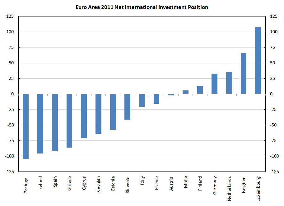
Here’s via Eurostat

It is clear from the chart that nations with high negative NIIP (and hence high net indebtedness) were/are the ones in trouble.

The accounting identity which connects the NIIP to CAB is:

Δ NIIP = CAB + Revaluations

Most of the times, revaluations have less of a role in explaining the NIIP. Of course one can always come up with exceptions – such as for the United States with huge revaluations due to outward FDI and Ireland. It should however be noted that Ireland also had high current account deficits.

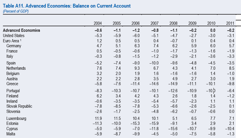
Here is data from the IMF on the current account balances:

From this you can see “Germany is not Greece”, “Netherlands is not Spain”, “Finland is not Cyprus” and so on and also the relation of CAB to NIIP.

Let me turn now to what Wray has to say:

Yesterday one presenter at this conference provided a lot of interesting data on cross border lending by European banks, most of which consisted of lending to fellow EMU members. He showed a strong correlation between cross border lending and cross border trade. Hence, posited a link between flows of finance and flows of goods and services. So far, so good. He also accepted a comment from the audience that correlation doesn’t prove causation, and that flows of finance are orders of magnitude larger than trade in goods and services—in other words, most of the financial churning has nothing to do with “real” production.

So atleast Wray accepts there is a correlation of some kind. For causation, see the arguments presented at the beginning of this post.

I won’t rehash that argument. Balances do balance, after all. For every current account deficit there’s a capital account surplus. It seems to me that the claim that the EMU suffers from “imbalances” is on even shakier ground. After all, they all use the same currency, so there’s no chance that an “imbalance” will lead to a run on the currency and to exchange rate depreciation (a usual fear following on from a current account deficit).

This argument was made by neoclassical economists around late 80s and early 90s when Europe was planning to form a monetary union. See this post Martin Wolf Pays A Generous Tribute To Anthony Thirlwall. Wray misses the point that a balance-of-payments crisis also leads to a deflationary spiral and that even though there is no exchange rate collapse, there is deflation in the Euro Area – exactly as predicted by those economists who thought the notion “current account deficits do not matter” was precisely wrong in the early 1990s.

Then Wray goes on to suggest that banks creating a boom and bust in Germany would have looked different:

Yes. But in what sense is that an “imbalance”? Look at it this way. What if instead of running up real estate prices in the sunny south—so that Brits and northern Europeans could enjoy vacation homes—the German banks had instead fueled a real estate bubble in Berlin? What if they had eliminated all underwriting standards and lent until the cows come home on the prospect that Berlin house prices would rise at an accelerating pace? Speculators from across the world would buy a piece of the bubble on the prospect that they’d reap the gains and sell-out at the peak. Construction activity would boom, workers could demand higher wages and would increase consumption, and Germany would have experienced higher price inflation than the rest of Euroland.

In the hypothetical case of Wray where German banks lend the non-financial sectors till the “cows come home”, domestic demand would have risen sharply (which he himself suggests) and this would have had the adverse effect on the balance of payments. Germany would have started running current account deficits because imports are dependent on domestic demand. Germany would have suffered similar fate but in the end it would have depended on how fast the domestic demand rose.

Wray should be careful in doing sectoral balances.

Bad bank behavior can boom or bust an economy—with or without current account deficits. And that’s pretty much what happened in Spain and Ireland (and also in Iceland).

Wray would have sounded right if he had given examples of nations having current account surpluses but from IMF’s table above it can be seen that both Spain and Ireland had huge current account deficits.

What about Iceland?

The data is from 2004-2011 and you can see that in 2008, Iceland had a current account deficit of 28.4%.

Wray then compares the Euro Area to the United States:

In Euroland, all use the same euro currency, and clearing is accomplished among the central banks and through the ECB (that is where Target 2 comes in). It works about as smoothly as the US system. But here’s the difference: the ECB “district banks” are national central banks. It is thus easier to keep mental tabs on the “imbalances” by member states in the EMU than in the USA.

Yes keeping mental tabs on imbalances (and not “imbalances”) can have its effect, but Wray crucially misses the point that in the United States, there is an automatic mechanism of compensating for trade imbalances via fiscal transfers. This acts via lower total taxes paid by regions facing slowdown caused by trade imbalances (not to be confused with lesser taxes paid due to reduced tax rates if any). A rise in public expenditure (not necessarily discretionary but resulting from government guarantees made beforehand) also helps.

Wray however quotes Mosler but he misses the point as well since it talks of directed government spending as opposed to a built in automatic mechanism which (the latter) prevents a crisis at this scale/type from happening.

Generally speaking, Wray seems to suggest that the crisis happened because the private sector credit-led boom went bust and this has nothing to do with current account imbalances. While it is true that the private sector credit-led boom ended in a bust and caused a crisis, what Wray misses is that the current account deficits contributed to exacerbating the crisis because nations in trouble built up huge indebtedness to the rest of the world and had troubles to refinance their debts. If all sectors of an economy have a consolidated net indebtedness position to the rest of the world, they will have issues borrowing and refinancing since – as a matter of accounting – foreigners have to attracted. Foreigners were unwilling because of doubts and also because there was/is a crisis in the world economy, they changed their portfolio preferences – making the whole issue of financing even more difficult.

A Digression On TARGET2

It can be argued that since the TARGET2 mechanism has a stabilizer of some sort – that since the Eurosystem TARGET2 claims arising due to capital flight from the “periphery” is an accommodative item in the balance-of-payments, current account deficits shouldn’t have been an issue.

The error in this argument is that while it is true that capital flight is automatically financed by the resultant Eurosystem TARGET2 claims and that this is helpful, it depends on the hidden assumption that banks have unlimited/uncollaterilized overdrafts at their home central banks. We have seen in various scenarios – such as with procedures such as the Emergency Liquidity Assistance (ELA) – that banks in the “periphery” can either run out of sufficient collateral needed to borrow from their home NCB or have chances to run out of collateral. They hence need to attract funds from abroad. The nation as a whole is dependent on foreigners. Current account deficits are not self-financing.
Some Aspects Of Central Bank Behaviour

There was a discussion last week on a social network site on Basil Moore’s book Horizontalists And Verticalists. Someone mentioned he never knew anyone who owned a copy of the book! Lucky me.

I was browsing through my copy and came across this – which I thought I should quote on central bank “defensive behaviour”.

Actually, among Post-Keynesians, Alfred Eichner was the first to understand and highlight the “defensive” nature of central bank open market operations.

Outside PKE, it was a paper of Raymond E. Lombra and Raymond G. Torto titled Federal Reserve Defensive Behaviour And The Reverse Causation Argument which started analyzing the details of the Federal Reserve defensive behaviour and supported the theory of endogenous money on which economists such as James Tobin and Nicholas Kaldor were writing at the time. The term “defensive” was coined by Robert Roosa of the Federal Reserve in the book Federal Reserve Operations In The Money And Government Securities Markets originally written in 1956.

Recently central banks around the world have been doing a lot of things (“unconventional measures”) in trying to “boost” their economies – such as “large scale asset purchases” (QE). For some, recent central bank action is the natural way to start to understand monetary economics. For me, it is first important to understand what they did before the crisis to correctly understand what they have been doing and judge if their actions have any usefulness at all – on a case by case basis.

Anyways, here is from Basil Moore’s book (pages 97-99):

Open-market operations: defensive rather than dynamic?

According to the conventional story taught in most textbooks and worked through by students in countless T-account exercises, central bank open-market security purchases have expansionary effects on the money stock by raising the high-powered base. Central bank security sales conversely lower the high-powered base, and so operate to reduce the stock of money outstanding.

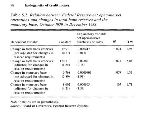
Table 5.2 presents the relationship between changes in total bank reserves, the monetary base, and the Federal Reserve net open-market security purchases or sales. The data are monthly time intervals for the period October 1979 to December 1983. This is the period when quantitative targeting was purportedly at last rigorously instituted. Nonborrowed reserves were avowedly the Fed’s chief operating instrument for controlling the growth rate of the monetary aggregates.

To the student of introductory economics, and even to many economists, these results will surely be startling. On a monthly basis, Federal Reserve net open-market operations fail to explain any of the actual changes in unadjusted or adjusted total reserves! They explain only 5 percent of changes in the unadjusted and only 10 percent of the changes in the high-powered base. In all cases the coefficient on net open-market purchases and sales is extremely small. It has no statistical significance in explaining observed changes in bank reserves. Although the coefficient is statistically significant in explaining the monetary base, its magnitude implies that $1000 of open-market purchases or sales were necessary to change the value of the base by $1!

The explanation for these apparently puzzling results is not far to seek (Lombra and Torto, 1973). From the central bank’s point of view a large number of stochastic nonpolicy factors operate to add or withdraw reserves from the banking system. These factors can be analyzed by an examination of the central bank’s balance sheet identity. This documents the various financial flows that accompany any change in the base: changes in float, changes in the public’s currency holding, foreign capital inflows or outflows, changes in treasury balances held with the Fed, changes in bank borrowing from the discount window. All of these flows are completely outside the control of the monetary authorities. In order to achieve a desired level of the base, these flows must be completely offset by open-market operations.

If the Fed were to take no action in the face of these large stochastic inflows and outflows of funds, the banking system would experience sharp fluctuations in its excess reserve position. Such changes would be unrelated to the Federal Reserve’s policy intentions, and would provoke continued liquidity crises and great instability in interest rates. As a result most Federal Reserve open-market operations are “defensive” and designed to offset the effects of these nonpolicy forces. Central banks operate to make reserves available to the banking system on reasonably stable terms, from day to day and week to week.

Studies of Federal Reserve open-market operations have estimated that more than 85 per cent of Federal Reserve security purchases of [sic] sales are “defensive” (Lombra and Torto, 1973, Forman, Groves and Eichner, 1984). Such flexibility is needed to deal with the very large inherent volatility of money flows. On a week-to-week basis such “noise” in the behaviour of the narrow money supply accounts for dollar changes in reserves of plus or minus $3 billion more than two-thirds of the time. This represents nearly 10 percent of total reserves, which were concurrently in the order of $40 billion (J. Pierce, 1982). On a monthly bias, such “noise” accounts for changes in the money stock or plus or minus 5 percent about two-thirds of the time.

Money And Shoes

… Now let me give you a ridiculous example to make the point. Don’t take it too seriously. Suppose that some statistician observes that over a long period of time there is a high association, a very good fit, between gross national product and the sales of, let us say, shoes. And then suppose someone comes along and says, “That’s a very good relationship. Therefore, if we want to control GNP, we ought to control production of shoes. So, henceforth, we’ll make shoes grow in production precisely at 4 percent per year, and that will make GNP do the same.” I don’t think you would have much confidence in drawing this second conclusion and policy recommendations from the observed empirical association.

Over the years, according to the monetarists, the Federal Reserve has been acting like the producers and sellers of shoes. That is, the Fed has been supplying money on demand from the economy instead of using the money supply to control the economy. The Fed has looked at the wrong targets and the wrong indicators. As a result, the Fed has allowed the supply of money to creep up when the demand for money rose as a result of expansion in business activity, and to fall when business activity has slacked off. This criticism implies that the supply of money has, in fact, not been an exogenously controlled variable over the period of observation. It has been an endogenous variable, responding to changes in economic conditions and credit market indicators via whatever response mechanism was built into the men in this room and their predecessors.

… Perhaps the monetarists will be sufficiently persuasive of the Federal Reserve and of Congressional committees to bring about, in the future, a controlled experiment in which the stock of money is actually an exogenous variable.

– James Tobin, 1969

Ref:

  1. Tobin, James, “The Role of Money In National Economic Policy – A Panel Discussion,” in Controlling Monetary Aggregates. Boston: Federal Reserve Bank of Boston, 1969, pp. 21-24 (link)

Income = Expenditure!

The accounting identities equating aggregate expenditures to production and of both to incomes at market prices are inescapable, no matter which variety of Keynesian or classical economics you espouse. I tell students that respect for identities is the first piece of wisdom that distinguishes economists from others who expiate on economics. The second?… Identities say nothing about causation.

– James Tobin

In my previous post Income ≠ Expenditure?, I raised some accounting issues in a recent talk by Steve Keen. I found a paper European Disunion and Endogenous Money which has a background on this written with Matheus Grasselli of the Fields Institute, Toronto.

Let us look at their basic model which still has income not equal to expenditure. Now whichever way one presents it (with better defined terms using phrases “ex-ante”, “ex-post”, “planned”, “unplanned”, one cannot escape the conclusion income = expenditure).

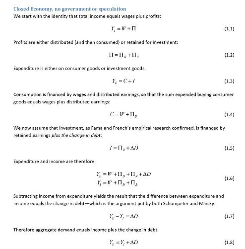
The model is below – found on page 15.

Keen has a simple two-sector model of households and production firms and it can also be thought of as a three sector model where production firms borrow from banks to finance investments.

In the last equation, you see Keen and Grasselli’s claim that expenditure is income plus change in debt.

The trouble is with Keen’s behavioural assumption (1.4)

C = W + Π

Unfortunately the rules of accounting do not allow this!

If the assumption (1.4) is relaxed, firms’ increase in debt is mirrored by households’ saving.

In a three sector model with households, firms and banks, the increase in firms’ debt is mirrored as increase in households’ deposits.

It can be generalized with firms issuing some securities purchased by households.

So equation 1.8 should read:

YE = Y

with no need of Lebesgue Integrals to prove (1.8) is correct because it is not correct.

The Saving = Investment Identity

The Keen-Grasselli model doesn’t respect the identity

Saving = Investment

This can be easily seen. Households (in his language workers) having zero saving and zero investment. Firms have a saving of  ΠR  and investment of I.

So total saving = Πand total investment = I

But because these terms differ by ΔD (equation 1.5), they cannot be equal unless ΔD = 0.

So in the Keen-Grasselli model,

Saving ≠ Investment

The reason Keen and Grasselli get this inconsistency is because they assume that saving is volitional.

Basil Moore was aware of this and in his book Shaking The Invisible Hand, he wrote:

The belief that aggregate saving is the sum of volitional saving decisions by individual economic units is simply a spectacular macroeconomic illustration of the “fallacy of composition.” This fallacy has been reinforced by the unfortunate use of the colloquial verb “to save,” with its very powerful transitive volitional connotations, for an economic term which is merely an intransitive accounting definition: “income not consumed.” As economists know, it is a “fallacy of composition” that what is true for the part is necessarily also true for the whole. Total “saving” is the sum of total saving undertaken by individual “savers.” But since saving is the accounting record of investment it cannot be the sum of volitional individual saving decisions. Aggregate saving is not the sum of individual savers volitional decisions to save. It follows that in all monetary economies most “saving” is “non-volitional.”

[emphasis: mine]

Ideally (i.e., realistically) Keen’s model should sit inside a model with the government and the government would end up running surpluses. Non-volitonally 🙂 S = I would be maintained and so would Y= Y

Some Higher Mathematics: The Dirac Delta Function

Keen and Grasselli claim that confusions around economists being not able to see things in continuous time is the source of errors by them and that the reason is that debt injections are sudden.

Now, in calculus, there is a thing called the Dirac Delta Function.

[Paul Dirac didn’t get the media attention that Einstein got but he was surely his equivalent. The Delta function is just a small contribution when compared to what he did elsewhere. He was Feynman’s hero.]

The delta function δ(x) is zero at all points except 0 where it is infinite. But the integral of δ(x) from over the range of real numbers is 1. That is difficult to digest initially when first tries to learn it.

A debt injection is a step function jump in debt. The delta function has a curious property that it is the derivative of the step function.

So income flows can be represented as sum of delta functions which different coefficients at different points in time.

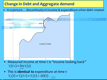
So Keen’s chart (Figure 13) in his paper should have income represented as delta function spikes.

To get the flow over a period, one has to integrate and this will result in the income over the period to be the sum of the coefficients of these delta functions.

So whether in discrete formulation or continuous time formulation, Y= Yfor the whole economy and the reason is not hard to guess because dD/dt cancels out with dA/dt since assets and liabilities are created equally.

For an individual sector it is true that Y= Y + dD/dt – nobody disagrees with that but to be more accurate the right hand side should include minus dA/dt.

Also, a continuous time formulation is just taking infinitesimal intervals and then treating infinite of them together.

It makes no sense to say income before debt injection was $100 for real world transactions in a continuous time formulation. It is actually zero just before a debt injection because all income/expenditure flows are “spikey”.

Just after the debt injection it is zero again because nobody spends the instant a loan is given. The debt injection increases assets and liabilities by the amount of the loan if the borrowing is from a bank.

So after the loan is given at the next infinitesimal, change in debt is zero and income/expenditure is also zero.

Then income/expenditure flow spikes at the moment the transaction happens – like a delta function.

But that is income for someone and for an economy as a whole Income = Expenditure.

Anyway, nothing of the analysis justifies the definition of “aggregate demand” (now renamed by Keen to “effective demand”).

20 Years Of Maastricht And All That

I recite all this to suggest, not that sovereignty should not be given up in the noble cause of European integration, but that if all these functions are renounced by individual governments they simply have to be taken on by some other authority. The incredible lacuna in the Maastricht programme is that, while it contains a blueprint for the establishment and modus operandi of an independent central bank, there is no blueprint whatever of the analogue, in Community terms, of a central government. Yet there would simply have to be a system of institutions which fulfils all those functions at a Community level which are at present exercised by the central governments of individual member countries.

The counterpart of giving up sovereignty should be that the component nations are constituted into a federation to whom their sovereignty is entrusted. And the federal system, or government, as it had better be called, would have to exercise all those functions in relation to its members and to the outside world which I have briefly outlined above.

That was published 8th October 1992 – exactly 20 years back!

Worth your time if you haven’t read it yet. Even if you have, worth reading it again!

Here’s the link to the full article Maastricht And All That by Wynne Godley.

Wynne Godley

(photo credit: King’s College, Cambridge)

Also check out John Cassidy’s post The Man Who Saw Through The Euro written for The New Yorker last year.

Income ≠ Expenditure?

I like Steve Keen. He is terrific in debunking economics! In a recent debate with Paul Krugman, Keen put Krugman on the defensive and exposed his weaknesses. Krugman obviously didn’t want to accept defeat and tried to escape with the help of comments in the comments section of Nick Rowe’s blog (that DSGE is not neoclassical – whatever!).

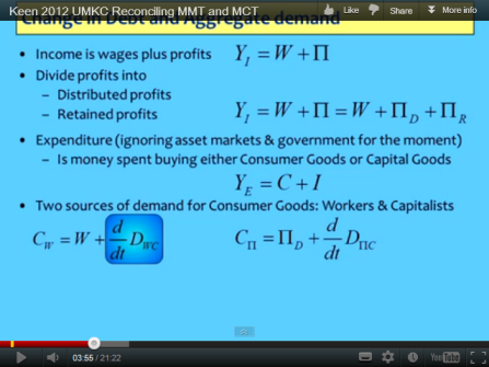
There are however some issues with Keen’s own methodologies. In a recent talk (video here), he claims that income is not equal to expenditure due to debt creation. Keen also claims in the video that Schumpeter and Minsky claimed that is the case.

Keen is right about an individual sector but not an economy as a whole when it is closed.

In the following I assume a closed economy – as does Keen. At least he doesn’t make any distinction and thereby his claim is a claim for a closed economy as well. So here is Keen’s claim:

Further he attributes this difference to discontinuities due to debt injections.

In the above Keen forgets that expenditure creates income.

There is no need for a claim that income is not equal to expenditure. In fact it is convenient to have them equal.

Wynne Godley and Francis Cripps wrote a nice book in 1983 named Macroeconomics. Here is from just the second page of Chapter 1: National Accounts:

It is extremely useful to choose definitions such that total income and expenditure in any year, month, day or second are identically equal to one another; they will be – because we choose to define them so that they are – two different ways of looking at the same process. We are only going to admit into the category of flows called income things which have an exact counterpart in the category of flows called expenditure. [footnote]

(with a footnote on qualifications for the case of an open economy).

Further in pages 27-29:

Although the definitions so far imply that the income of all individuals and institutions taken together equals their total expenditure on goods and services in each and every period, this need not be true of any particular person or institution …

… It is easy to understand that any one individual who does not spend all his or her income in a period will have more money left over at the end of the period. But we have chosen a system of definitions which ensures that total income in each period when summed across the whole economy equals total expenditure in the same period. It must therefore be the case that if some people or institutions are accumulating money or other financial assets, others are incurring debts on an exactly equal scale. In the economy as a whole the total increase in financial assets must always be equal in each period to the total increase in debt (financial liabilities).

But since the possibility of borrowing is included as a source of funds for spending, our formal representation of the budget constraint for any individual or institution including the government, is

Equation 1.4 simply says that any excess of income over spending must equal the acquisition of financial assets less the acquisition of debts. As this is true for all individuals it must also be true for the economy as a whole.

But since total national income equals total national expenditure (i.e., Y ≡ E) it must follow for the economy as a whole the change in financial assets must be equal to the aggregate change in debt, i.e.,

ΔFA ≡  ΔD

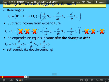
Back to Keen. He has this slide in this talk:

In the above, households consume by getting wages and going into debt. Hence households have their expenditure higher than income. Similar story for firms.

However, Keen forgets that consumption is income for firms and his accounting has black holes. The whole thing can be done right by creating a Transactions Flow Matrix, so that one is sure that nothing is missed out.

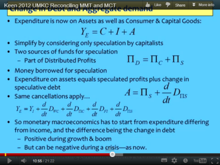
The reason Keen gets into paradoxes can be seen by looking at the following slide where he changes the definition of expenditure.

The right definition of expenditure does not include purchases of financial assets. For Keen if  a household purchases financial assets, it will be counted as “expenditure”. From the above slide, it can be seen that Keen’s definition of expenditure itself is different to begin with from standard ones and obviously he gets the paradoxical claim that Income ≠ Expenditure!

If Keen wants to do an empirical study of the rise in gross assets and liabilities, there is a systematic way to do this: for example see this Bank of England paper Growing Fragilities – Balance Sheets In The Great Moderation.

I won’t pursue this further except saying a few things.

I think Keen’s intuition is that households and firms incurred liabilities at an increasing scale before the financial crisis for both expenditures and purchases of financial assets and this led to increases in asset prices and hence capital gains and hence a feedback loop leading to debt-fuelled growth. Etc etc etc. There is a way to do this but changing definitions is not the right way.

Keen’s model will look accounting consistent (highly important) and more realistic (with no need to define aggregate demand = gdp + change in debt) if he uses some sort of econometric modeling in which Private Expenditure PX is dependent on many things – for example PX-1 so that income need not be equal to expenditure for the economy as a whole (as the time periods for which they are recorded are different) and there is some sort of econometric relation with change in debt.

Else one gets hodgepodge and/or endless redefinitions.

I think his “model” mixes identities, behaviour and plausible econometric relationships.

Below are some “endnotes”

Change in Inventories

“Change in Inventories” create some issues for “Y ≡ E”.  The right way is to have Expenditure equal Final Purchases plus change in inventories. As per Godley & Cripps (p 33):

Y ≡ E = FE + ΔI

Open Economies

Funnily, it is in the case of an open economy that for an economy as a whole, Income ≠ Expenditure! The difference between expenditure and income is equal to the increase in net indebtedness to foreigners.

GDP by Expenditure

Expenditure (of a resident sectors) used here shouldn’t be confused with the expenditure in “gdp by expenditure”. In the former, we include expenditures of residents while in the latter, the export component refers to expenditure of the rest of the world sector of goods and services produced by resident sectors.