Yearly Archives: 2012

Income And Expenditure Flows And Financing Flows

In the previous two posts, I went into a description of the transactions flow matrix and the balance sheet matrix as tools for an analytic study of a dynamical study of an economy.

During an accounting period, sectors in an economy are making all kinds of transactions. These can be divided into two kinds:

  1. Income and Expenditure Flows
  2. Financing Flows

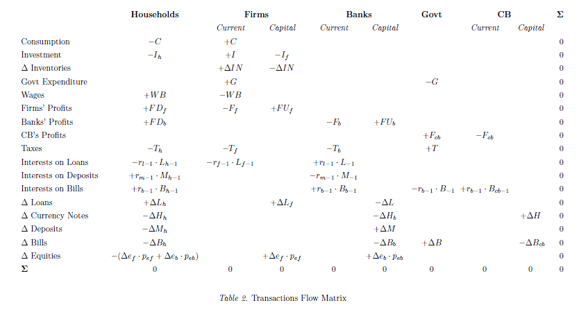
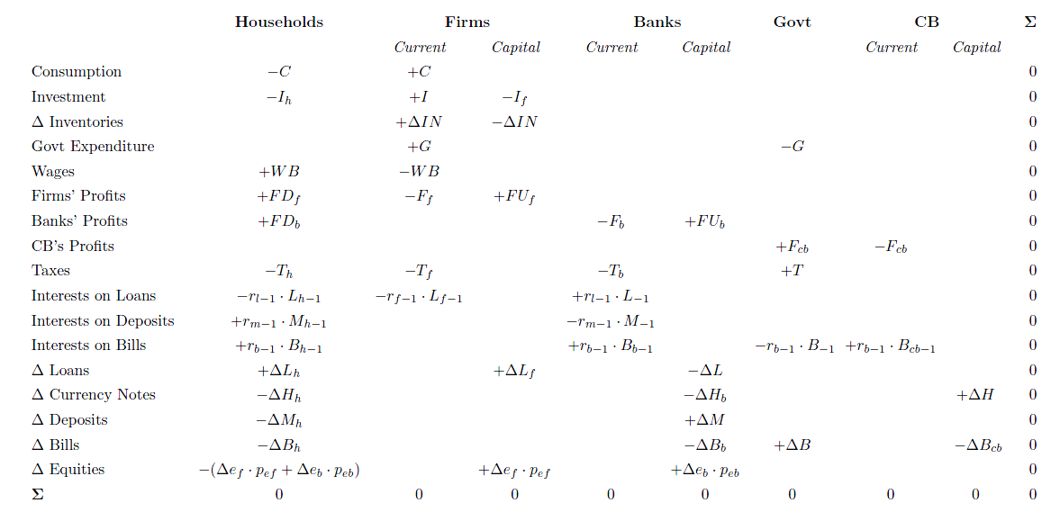
Let’s have the transactions flow matrix as ready reference for the discussion below.

(Click for a nicer view in a new tab)

The matrix can easily be split into two – on top we have rows such as consumption, government expenditure and so on and in the bottom, we have items which have a “Δ” such as “Δ Loans” or “change in loans”. We shall call the former income and expenditure flows and the latter financing flows.

To get a better grip on the concept, let us describe household behaviour in an economy. Households receive wages (+WB) and dividends from production firms (called “firms” in the table) and banks (+FD_{f} and +FD_{b}) respectively) on their holdings of stock market equities. They also receive interest income from their bank deposits and government bills. These are sources of households’ income. While receiving income, they are paying taxes and consuming a part of their income (and wealth). They may also make other expenditure such as buying a house or a car. We call these income and expenditure flows.

Due to these decisions, they are either left with a surplus of funds or a deficit. Since we have clubbed all households into one sector, it is possible that some households are left with a surplus of funds and others are in deficit. Those who are in surplus, will allocate their funds into deposits, government bills and equities of production firms and banks. Those who are in deficit, will need funds and finance this by borrowing from the banking system. In addition, they may finance it by selling their existing holding of deposits, bills and equities. The rows with a “Δ” in the bottom part of transactions flow matrix capture these transactions. These flows will be called financing flows.

How do banks provide credit to households? Remember “loans make deposits”. See this thread Horizontalism for more on this.

This can be seen easily with the help of the transactions flow matrix!

The two tables are some modified version of tables from the book Monetary Economics by Wynne Godley and Marc Lavoie.

It is useful to define the flows NAFA, NIL and NL – Net Accumulation of Financial Assets, Net Incurrence of Liabilities and Net Lending, respectively.

If households’ income is higher than expenditure, they are net lenders to the rest of the world. The difference between income and expenditure is called Net Lending. If it is the other way around, they are net borrowers. We can use net borrowing or simply say that net lending is negative. Now, it’s possible and typically the case that if households are acquiring financial assets and incurring liabilities. So if their net lending is $10, it is possible they acquire financial assets worth $15 and borrow $5.

So the the identity relating the three flows is:

NL = NAFA – NIL

I have an example on this toward the end of this post.

I have kept the phrase “net” loosely defined, because it can be used in two senses. Also, some authors use NAFA when they actually mean NL – because previous system of accounts used this terminology as clarified by Claudio Dos Santos. I prefer old NAFA over NL, because it is suggestive of a dynamic, though the example at the end uses the 2008 SNA terminology.

While households acquire financial assets and incur liabilities, their balance sheets are changing. At the same time, they also see holding gains or losses in their portfolio of assets. What was still missing was a full integration matrix but that will be a topic for a post later. Since, it is important however, let me write a brief mnemonic:

Closing Stocks = Opening Stocks + Flows + Revaluations

where revaluations denotes holding gains or losses.

This is needed for all assets and liabilities and for all sectors and hence we need a full matrix.

We will discuss more on the behaviour of banks (and the financial system) and production firms some other time but let us briefly look at the government’s finances.

As we saw in the post Sources And Uses Of Funds, government’s expenditure is use of funds and the sources for funds is taxes, the central bank’s profits, and issue of bills (and bonds). Unlike households, however, the government is in a supreme position in the process of “money creation”. Except with notable exceptions such as in the Euro Area, the government has the power to make a draft at the central bank under extreme emergency, though ordinarily it is restricted. Wynne Godley and Francis Cripps described it as follows in their 1983 book Macroeconomics:

Our closed economy has a ‘central bank’ with two principle functions – to manage the government’s debt and to administer monetary policy. [Footnote: The central bank has to fund the government’s operations but this in itself presents no problems. Government cheques are universally accepted. When deposited with commercial banks the cheque become ‘reserve assets’ in the first instance; banks may immediately get rid of excess reserve assets by buying bonds.]. The only instrument of monetary policy available to the central bank in our simple system is the buying and selling of government bonds in the bond market. These operations are called open market operations. We assume that the central bank does not have the right to directly intervene directly in the affairs of commercial banks (e.g., to prescribe interest rates or quantitative lending limits) or to change the 10% minimum reserve requirement. But the central bank is in a very strong position in the bond market since it can sell or buy back bonds virtually without limit. This gives it the power, if it chooses, to fix bond prices and yields unilaterally at any level [Footnote: But speculation based on expectations of future yields may oblige the central bank to deal on a very large scale to achieve this objective.] and thereby (as we shall soon see) determine the general level of interest rates in the commercial banking system.

Given such powers, we can assume in many descriptions that the government’s expenditure and the tax rate is exogenous. However, many times, there are many constraints such as price and wage rises, high capacity utilization and low production capacity and also constraints brought about from the external sector due to which fiscal policy has to give in and become endogenous.

While I haven’t introduced open economy macroeconomics in this blog in a stock-flow coherent framework, we can make some general observations:

For a closed economy as a whole, income = expenditure. While it is true for the whole economy (worth stressing again: closed), it is not true for individual sectors. The household sector, for example, typically has its income higher than expenditure. In the last 15-20 years, even this has not been the case. If one sector has it’s income higher than expenditure, some sectors in the rest of the world will have its income lower than its expenditure. Many times, the government has its income lower than expenditure and we see misleading public debates on why the government should aim to achieve a balanced budget. When a sector has its income lesser than expenditure, it’s net lending is negative and hence is a net borrower from the rest of the world. It can finance this by borrowing or sale of assets. A region or a whole nation can have its expenditure higher than income and this is financed by borrowing from the rest of the world. A negative flow of net lending implies a net incurrence of liabilities – thus adding to the stock of net indebtedness which can run into an unsustainable territory. Stock-flow coherent Keynesian models have the power to go beyond short-run Keynesian analysis and study sustainable and unsustainable processes.

In an article Peering Over The Edge Of The Short Period – The Keynesian Roots Of Stock-Flow Consistent Macroeconomic Models, the authors Antonio C. Macedo e Silva and Claudio H. Dos Santos say:

… it is important to have in mind that it is possible to get three kinds of trajectories with SFC models:

  • trajectories toward a sustainable steady state;
  • trajectories toward a steady state over certain limits;
  • explosive trajectories.

The analysis of SFC models’ dynamic trajectories and steady states is useful, first because it makes clear to the analyst whether the regime described in the model is sustainable or whether it leads to some kind of rupture—either because the trajectory is explosive or because it leads to politically unacceptable configurations. In these cases, as Keynes would say in the Tract, the analyst can conclude that something will have to change and even get clues about (i) what will probably change (since the sensitivity of the system dynamics to changes in different behavioural parameters is not the same); and (ii) when this change will occur (since the system may converge or diverge more or less rapidly).

Example

Note that Net Lending is different from “saving”. Say, a household earns $100 in a year (including interest payments and dividends), pays taxes of $20 and consumes $75 and takes a loan of to finance a house purchase near the end of the year whose price is $500. Assume that the Loan-To-Value (LTV) of the loan is 90% – which means he gets a loan of $450 and has to pay the remaining $50 from his pocket to buy the house. (i.e., he is financing the house mainly by borrowing and partly by sale of assets). How does the bank lending – simply by expanding it’s balance sheet (“loans make deposits”). Ignoring, interest and principal payments (which we assume to fall in the next accounting period),

His saving is +$100 – $20 – $75 = +$5.

His Investment is +$500.

His Net Incurrence of Liabilities is +$450.

His Net Accumulation of Financial Assets is +$5 – $50 = – $45.

His Net Lending is = -$45 – (+$450) = -$495 which is Saving net of Investment ($5 minus $500).

This means even though the person has “saved” $5, he has incurred an additional liability of $450 and due to sale of assets worth $45, he is a net borrower of $495 from other sectors (i.e., his net lending is -$495).

Assume he started with a net worth of $200.


Opening Stocks: 2010

$

Assets

200

Nonfinancial Assets
Deposits
Equities

0
30
170

Liabilities and Net Worth

200

Loans
Net Worth

0
200


Now as per our description above, the person has a saving of $5 and he purchases a house worth $500 by taking a loan of $450 and selling assets worth $50. We saw that the person’s Net Accumulation of financial assets is minus $45. How does he allocate this? (Or unallocate $45)? We assume a withdrawal of $10 of deposits and equities worth $35. At the same time, during the period, assume he had a holding gain of $20 in his equities due to a rise in stock markets.

Hence his deposits reduce by $10 from $30 to $20. His holding of equities decreases by $15 (-$35 + $20 = -$15)

How does his end of period balance sheet look like? (We assume as mentioned before that the purchase of the house occurred near the end of the accounting period, so that principal and interest payments complications appear in the next quarter.)


Closing Stocks: 2010

$

Assets

675

Nonfinancial Assets
Deposits
Equities

500
20
155

Liabilities and Net Worth

675

Loans
Net Worth

450
225


Just to check: Saving and capital gains added $5 and $20 to his net worth and hence his net worth increased to $225 from $200.

Of course, from the analysis which was mainly to establish the connections between stocks and flows seems insufficient to address what can go wrong if anything can go wrong. In the above example, the household’s net worth gained even though he was incurring a huge liability. What role does fiscal policy have? The above is not sufficient to answer this. Hence a more behavioural analysis for the whole economy is needed which is what stock-flow consistent modeling is about.

One immediate answer that may satisfy the reader now is that the households’ financial assets versus liabilities has somewhat deteriorated and hence increased his financial fragility. By running a deficit of $495 i.e., 495% of his income, the person and his lender has contributed to risk. Of course, this is just one time for the person – he may be highly creditworthy and his deficit spending is an injection of demand which is good for the whole economy. After all, economies run on credit. While this person is a huge deficit spender, there are other households who are in surplus and this can cancel out. In the last 15 years or so, however (before the financial crisis hit), households (as a sector) in many advanced economies ran deficits of the order of a few percentage of GDP. If the whole household sector continues to be a net borrower for many periods, then this process can turn unsustainable as the financial crisis in the US proved.

Now to the title of the post. Flows such as consumption, taxes, investment are income/expenditure flows. Flows such as “Δ Loans”, “Δ Deposits”, “Δ Equities” are financing flows. Income/expenditure flows affect financing flows which then affect balance sheets, as we see in the example.
Net Worth

In my previous post Sources And Uses Of Funds, I used the term “net worth”, and the reader would have noted the the strange dissimilarity with business accounting.

It’s best first to verify that national accountants (with the exception of the Federal Reserve’s Z.1 flow of funds accounts of the United States) do it the way described in the previous post.

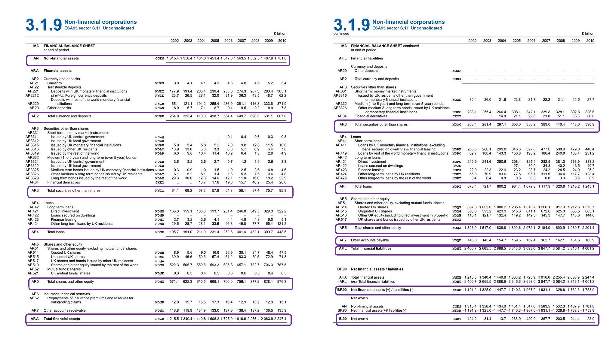
The UK Blue Book 2011 has the following description of Non-financial corporations’ balance sheet at the end of 2010:


Assets

Nonfinancial Assets
Currency and Deposits
Securities Other Than Shares
Loans
Shares and Other Equity
Other Accounts Receivable

Liabilities and Net Worth

Currency and Deposits
Securities Other Than Shares
Loans
Shares and Other Equity
Other Accounts Payable
Net Worth

£,  billion

4,029.2

1,781.8
687.8
85.3
448.5
876.8
135.9

4,029.2


390.9
1,245.1
2,201.4
163.9
28.0


The relevant tables are below:

So “Shares and Other Equity” is treated as a liability of the corporation even though dividends are not compulsory. In a sense, equities are treated as being equivalent to debt securities. How does one calculate this? Assuming the relevant information is available, one simply needs to calculate the market value of equities issued by corporations.

The tendency to treat equities issued by corporations as not liabilities is misleading. This is all the more important if foreigners hold a large amount of equities and this may underestimate the indebtedness to foreigners. Indeed statistical agencies of many nations release data for the loosely defined term “external debt” and do not count equities held by foreigners in this. This “intuition” can easily be dismissed – foreigners can liquidate equities.

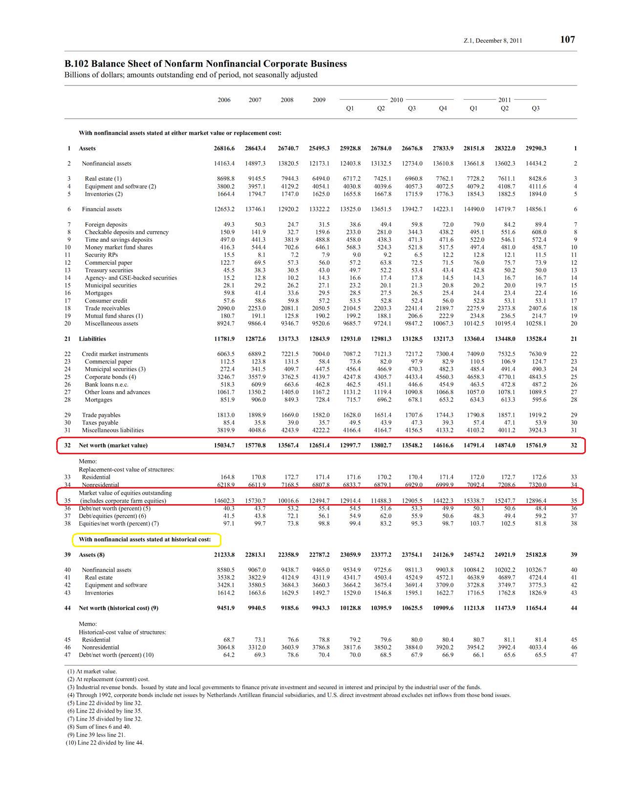
For comparison, below is the similar Z.1 statistic of Nonfarm Nonfinancial Corporate Businesses of the United States

The Federal Reserve by excluding the market value of equities issued in liabilities, exaggerates the net worth of corporations.

SNA Description of Differences

The System of National Accounts describes the differences in Section 1.64

Business accounts commonly (but not invariably) record costs on an historic basis, partly to ensure that they are completely objective. Historic cost accounting requires goods or assets used in production to be valued by the expenditures actually incurred to acquire those goods or assets, however far back in the past those expenditures took place. In the SNA, however, the concept of opportunity cost as defined in economics is employed. In other words, the cost of using, or using up, some existing asset or good in one particular process of production is measured by the amount of the benefits that could have been secured by using the asset or good in alternative ways. Opportunity cost is calculated with reference to the opportunities foregone at the time the asset or resource is used, as distinct from the costs incurred at some time in the past to acquire the asset. The best practical approximation to opportunity cost accounting is current cost accounting, whereby assets and goods used in production are valued at their actual or estimated current market prices at the time the production takes place. Current cost accounting is sometimes described as replacement cost accounting, although there may be no intention of actually replacing the asset in question after it has been used.

So current cost accounting or replacement cost accounting is used. We saw in the last post that financial assets and liabilities are to be valued at their market values. In addition, real estate will be evaluated at the market price. Capital goods are to be valued at their replacement cost. Inventories should be valued at the current cost of production, not at the price the producers expect to it to sell.

Moreover, according to the SNA:

Current cost accounting has ramifications that permeate the entire SNA. It affects all the accounts and balance sheets and their balancing items. A fundamental principle underlying the measurement of gross value added, and hence GDP, is that output and intermediate consumption must be valued at the prices current at the time the production takes place. This implies that goods withdrawn from inventories must be valued at the prices prevailing at the times the goods are withdrawn and not at the prices at which they entered inventories. This method of recording changes in inventories is not commonly used in business accounting, however, and may sometimes give very different results, especially when inventory levels fluctuate while prices are rising. Similarly, consumption of fixed capital in the SNA is calculated on the basis of the estimated opportunity costs of using the assets at the time they are used, as distinct from the prices at which the assets were acquired. Even when the fixed assets used up are not actually replaced, the amount of consumption of fixed capital charged as a cost of production should be sufficient to enable the assets to be replaced, if desired. When there is persistent inflation, the value of consumption of fixed capital is liable to be much greater than depreciation at historic costs, even if the same assumptions are made in the SNA and in business accounts about the service lives of the assets and their rates of wear and tear and obsolescence. To avoid confusion, the term “consumption of fixed capital” is used in the SNA to distinguish it from “depreciation” as typically measured in business accounts.

Back to Net Worth

The SNA has this description of net worth:

Net worth is the difference between the value of all financial and non-financial assets and all liabilities at a particular point in time. For this calculation, each asset and each liability is to be identified and valued separately. As the balancing item, net worth is calculated for institutional units and sectors and for the total economy.

For government, households and NPISHs [Non-profit institutions serving households], the value of net worth is clearly the worth of the unit to its owners. In the case of quasi-corporations, net worth is zero, because the value of the owners’ equity is assumed to be equal to its assets less its liabilities. For other corporations, the situation is less clear-cut.

In the SNA, net worth of corporations is calculated in exactly the same way as for other sectors, as the sum of all assets less the sum of all liabilities. In doing so, the value of shares and other equity, which are liabilities of corporations, are included in the value of liabilities. Shares are included at their market price on the balance sheet date. Thus, even though a corporation is wholly owned by its shareholders collectively, it is seen to have a net worth (which could be positive or negative) in addition to the value of the shareholders’ equity.

Update: Corrected the values in the table at the beginning of the post.

Sources And Uses Of Funds

In a recent post, I went into what is called the Transactions Flow Matrix. This is used heavily in Stock-Flow Consistent Modeling of the whole economy. The underlying theme is “everything comes from somewhere and goes somewhere, and there are no black holes”.

I also mentioned about a Balance Sheet Matrix. What is it?

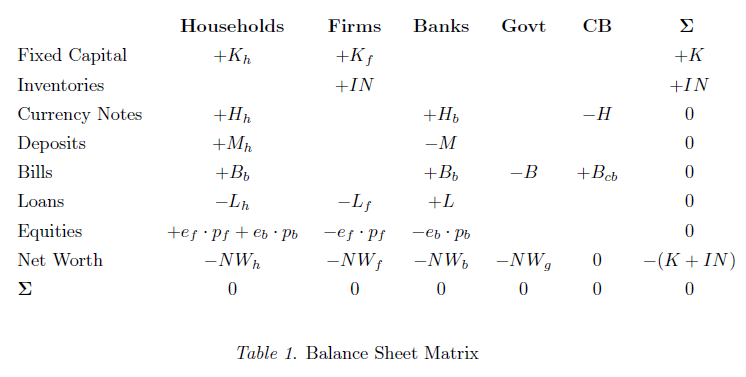
Sectors in an economy have assets and liabilities. Assets can be both financial as well as nonfinancial. Since nonfinancial assets are nobody’s liability, liabilities are financial. Very quickly, a balance sheet matrix is created by assigning a + sign to assets and a (-) sign to liabilities.

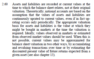
As per the System of National Accounts, all assets and liabilities are to be evaluated at market prices. According to 2008 SNA,

So a corporation or the government may have issued bonds at $100 but since the value fluctuates everyday and even during the day, it is possible that the bond price may reach $103. If it is the last day of the period for which the balance sheet is compiled, then the liability should be entered as $103, not $100.

We will have more to see in another post but let us just have a cursory look at an item called net worth. Since balance sheets should balance, we include this item in liabilities or rather call the right hand side of a balance sheet “Liabilities and Net Worth”. The term Net Worth has an intuitive appeal. If I have assets worth $100 and owe someone (say a bank) $10 and nothing more or less, my net worth is $90.

So let us quickly jump into the balance sheet matrix of a model economy.

In the previous post on the Transactions Flow Matrix, I had amalgamated the sectors Government and Central Bank into one, but now I have separated them so that there is higher clarity.

The reason I am writing this post is to stress the importance of signs. So in the above you will notice that households have a liability of L_{h} and hence appears with a negative sign. We shall see below however, that since loans are a source of funds, it will appear as a positive sign in the transactions flow matrix!

So households hold currency notes, deposits, bills and equities and these have counterpart in some other sector. And this should be the case because every financial asset is someone else’s liability. Also, from the matrix, the sum of net worths of all sectors (for a closed economy, at any rate) is equal to the value of the nonfinancial assets. This result isn’t surprising since financial assets cancel out with their counterpart liabilities.

We now jump to the transactions flow matrix – which I remade and added a lot of complications as compared to the previously related post The Transactions Flow Matrix

(Click to enlarge in a new tab)

These matrices are almost exactly similar to what appears in Wynne Godley and Marc Lavoie’s book Monetary Economics. 

The difference between the two matrices is that the balance sheet matrix records assets and liabilities at the beginning or the end of a period, whereas the transactions flow matrix records transactions during an accounting period.

In the previous post I had briefly stressed the importance of signs but now we have the balance sheet matrix as well ready, let me stress this again using a few lines from G&L’s book on the transaction flow matrix (page 40):

The best way to take it in is by first running down each column to ascertain that it is a comprehensive account of the sources and uses of all flows to and from the sector and then reading across each row to find the counterpart of each transaction by one sector in that of another. Note that all sources of funds in a sectoral account take a plus sign, while the uses of these funds take a minus sign. Any transaction involving an incoming flow, the proceeds of a sale or the receipts of some monetary flow, thus takes a positive sign; a transaction involving an outgoing flow must take a negative sign. Uses of funds, outlays, can be either the purchase of consumption goods or the purchase (or acquisition) of a financial asset. The signs attached to the ‘flow of funds’ entries which appear below the horizontal bold line are strongly counter-intuitive since the acquisition of a financial asset that would add to the existing stock of asset, say, money, by the household sector, is described with a negative sign. But all is made clear so soon as one recalls that this acquisition of money balances constitutes an outgoing transaction flow, that is, a use of funds.

So the government expenditure G has a minus sign because it is a use of funds and its sources are taxes, net issuance of bills and central bank profits.

The sources of funds for the production sector (abbreviated “firms”) is retained earnings (or undistributed profits, called FU), loans from banks and the issuance of equities and also sales (the consumption by households), government purchase of goods and investment itself because producers create tangible capital for themselves as a whole.

Now compare signs in the two matrices – equities are a source of funds for firms and hence has a positive sign in the transactions flow matrix but equities are also liabilities and hence the stock of equities appears with a negative sign in the balance sheet matrix.

Similarly, borrowing via loans are a source of funds for households and hence the positive sign in Table 2 while in Table 1 it appears with a minus sign.

For banks, making loans is a use of funds and taking deposits a source of funds. Hence minus and plus respectively in Table 2.

Also, the equities and loans in Table 2 are flows whereas in Table 1 they are stocks. Hence in Table 2, we have “Δ Loans” or change in loans, whereas in Table 1 its simply “Loans”.

Once we have a beginning of period balance sheet matrix and the transactions flow matrix, how do we construct the end of the period balance sheet matrix? I will leave this question for another post because I will have to introduce capital/holding gains and something called a full integration matrix. Before that I will have another post on real numbers taken from statistical releases to get more a intuitive feel for the balance sheet matrix.

The three matrices (the transactions flow matrix, the balance sheet matrix and the full integration matrix) go into the heart of “how money is created”. For this to be seen in detail, I will have to go into “monetary circuits” using transaction flows and that is the topic of yet another post. If you really understand how loans make deposits, the two tables should set you into a dynamical view of the whole process – a description completely different than the chimerical money multiplier model.

Spam And ReCAPTCHA

I have added ReCAPTCHA for commenting, as I get too many spams from robots who tell me how wonderful my blog is.

I used ReCAPTCHA since it is maintained by Google and better than ones made with less effort.

The flip side is that sometimes the words do not appear very readable, so can you please reload using the reload button (circled in gray above) – if that’s the case.

As a reminder, I love getting comments but don’t publish them and interact with the commenters on email.

FX Turnover

The Bank of England and the Federal Reserve Bank of New York reported the results of their survey of the volume of activity in the foreign exchange markets today. (here and here).

According to the Bank of England,

Average daily reported UK foreign exchange turnover1 was $1,972 billion in October 2011, 3% lower than in April 2011, and 17% higher than a year earlier.

and according to the Federal Reserve,

Average daily volume in total over-the-counter foreign exchange instruments (including spot, outright forward, foreign exchange swap, and option transactions) reached a record high of $977 billion in October 2011, compared with upwardly revised turnover figures of $856 billion in April 20111 and $809 billion in October 2010. The October 2011 total represented a 14.2 percent increase from the prior survey.

The Bank of International Settlements releases its own survey – the difference between its survey and that of central banks’ is the BIS collects data from banks’ sales desks while the central banks collect data directly from the dealers’ trading desks. (Minor point)

Why is this so high? (As compared to transactions in goods and services)

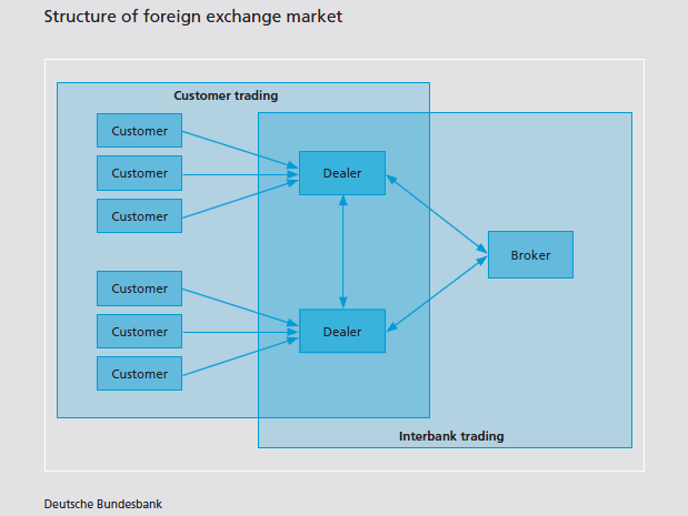
To understand this, we need to look at the mircostructure of the foreign exchange markets. Like all markets, the foreign exchange market has dealers and in this case its banks who make the markets.

Here’s a nice diagram from the Deutsche Bundesbank’s Monthly Report, January 2008

Two Way Quotes

Consider a EUR/USD quote such as 1.3063/1.3065.

buy/sell or bid/offer.

What does that mean?

If you as a customer (not the dealer) want to sell EUR, the dealer is bidding at $1.3063. That is, you enter into the transaction at this quote, you receive $1.3063 for every €1 you sell the dealer (dealer buys EUR). If you want to buy EUR, you pay $1.3065 for every €1 you purchase from the dealer (dealer sells EUR). The buy/sell is from the market maker’s perspective.

The quote (the spread actually) is always in the market maker’s favour because he/she runs the risk of a one-sided inventory.

Once the customer accepts the quote, the bank has “undesired” inventory. So it is looking to reduce this and needs another dealer who can be contacted through a broker or a broker’s trading system. Before the trade, the identity of the other side is confidential to the broker and is revealed after the trade is done because settlement has to take place. Unlike dealers, brokers do not take positions and receive a broker fee for the transactions they acted as brokers.

[In one of my future posts, I will cover settlements of international trades because I believe the concept of settlement goes into the heart of the question: What Is Money.]

This leads to a multiplier effect, since the second dealer also may have excess inventory and this explains the high turnover in the fx markets. In an article Mark Flood from the Federal Reserve Bank of St. Louis, Market Structure and Inefficiency in the Foreign Exchange Market, 1994, wrote:

The large volume of interbank trading is not primarily speculative in nature, but rather represents the tedious task of passing undesired positions along until they happen upon a marketmaker whose inventory discrepancy they neutralize.

The whole process is a bit haphazard way of shifting risk back to their customers!

Kaldorians

In an article (obituary), Nicholas Kaldor, 12 May 1908-30 September 1986, Geoff Harcourt said:

Nicholas Kaldor’ resembled Keynes more than any other twentieth-century economist because of the breadth of his interests, his wide-ranging contributions to theory, his insistence that theory must serve policy, his periods as an adviser to governments, his fellowship at King’s and, of course, his membership of the House of Lords.

I was reading this article (for the 3rd time!) Kaldor And The Kaldorians by John E. King. It appears as a chapter in the book Handbook Of Alternative Theories Of Economic Growth edited by Mark Setterfield.

I came across this strong Kaldorian view (which I share):

How, exactly, does the constraint [balance-of-payments constraint] operate? Three mechanisms can be distinguished. First, in extreme cases like Cuba in the 1990s and Zimbabwe in the 2000s, a shortage of foreign exchange makes it impossible fully to operate the existing capital stock (since spare parts can no longer be imported), and growth declines or becomes negative. Second, during the fixed exchange rate regime imposed by the Bretton Woods system (1945–73), governments were forced to implement deflationary monetary and fiscal policies to protect the currency in face of often quite small payments deficits. This generated the “stop–go” cycle that Kaldor regarded as the principal cause of Britain’s poor growth performance in this period. Third, in a floating exchange rate regime, the principal constraint on output growth is the rate of growth of export demand. Kaldor himself came to believe that exports were the only source of autonomous aggregate demand, since all other categories of expenditure were fully determined by income: consumption directly, investment indirectly through the accelerator coefficient, and government spending indirectly through taxation receipts, themselves a function of income. This is a characteristically extreme position, which is difficult to justify. But it is not necessary to deny the existence of some autonomous consumption, investment and government spending in order to recognise the importance of export demand as a factor in economic growth. For most small countries, and for all regions within countries, exports are indeed the most important factor.

I am not sure if King’s description of Kaldor and the Kaldorians is the best but a decent one. So, as King hints, Kaldor fully understood the injection to demand due to government expenditure and private sector borrowing. In fact, one whose views closely resembled that of Kaldor was Wynne Godley.

How are exports determined?

Nicholas Kaldor, Geneva, 1948

Picture source: Economica

Kaldor had the following to say:

The growth of a country’s exports should itself be considered as the outcome of the efforts of its producers to seek out potential markets and to adapt their product structure accordingly. Basically in a growing world economy the growth of exports is mainly to be explained by the income elasticity of foreign countries for a country’s products; but it is a matter of the innovative ability and adaptative capacity of its manufacturers whether this income elasticity will tend to be relatively large or small.

in “The role of Increasing Returns, Technical Progress and Cumulative Causation in the Theory of International Trade and Economic Growth”, Economie Appliquée, 1981

This is oft-quoted by economists who are inspired by Kaldor’s work. This may look straightforward but in my opinion, it is not so in practice. There are just too many different kinds of stories one hears about the external sector from economists. In stock-flow-consistent Post Keynesian macro modelling literature, one sees equations such as

The algebra is involved and there are many more equations than the above two. To get exports and imports, one has to multiply the x£ and im£ by prices. Refer Godley&Lavoie’s text Monetary Economics, oft referred in this blog.

The above equation assumes important causalities. Exports of a nation depends on prices of exported products relative to domestic prices of products in the foreign country, for example. In addition, exports also depend on demand and income in the foreign country(y$). The parameter ε2 (and μ2 from foreigners’ viewpoint) is what Kaldor is talking of in the quote above. The more competitive producers in the £-country are, the higher ε2 will be. Of course, this is not the only important thing, and prices are also important. (For example, if the GBP starts appreciating, UK exporters will face pressures in selling their products in the US).

The above equation also shows that if there are injections to demand, such as from government expenditure or tax cuts or due to higher private expenditure (either by higher borrowing or an increased propensity to consume etc), imports will increase. Similarly, if there is a contraction, imports will decrease as was evident by the collapse of world trade due to recessions in many parts of the world during the “Great Recession”.

The purpose of my post was to highlight what importance economists give to price-elasticity and income-elasticity of exports/imports. Most economists worry too much about ε1 (and μ1) and Kaldorians pay much more attention to ε2 (and μ2) and what sorts of policies governments should follow based on this. For example, a nation’s government may be concentrating too much in promoting exports of goods and services where price-competitiveness plays a role. It may be beneficial if it switches to promoting exporting goods and services in which it has unique capabilities which if successful will greatly improve its external situation.

In fact, according to the work of Kaldorians such as Anthony Thirwall and John McCombie, growths of nations can be explained by the ratio of the rate of growth of exports to the income elasticity of its imports. In the stronger form, exports themselves depend on the income-elasticity of imports in the foreign nation – i.e., the “non-price competitiveness” of exporters.

The two authors wrote an excellent book in 1994: Economic Growth And The Balance-Of-Payments Constraint – considered one of the greatest books in Post-Keynesian Economics.

The (Almost) Irrelevance Of Reserve Requirements

Earlier this week, the Reserve Bank of India reduced banks’ reserve requirements by 50bps. It’s called Cash Reserve Ratio and the RBI reduced it from 6.00% to 5.50% with effect from the following week.

The Reserve Bank of India is one of the most backward central bank in liquidity management and sometimes panics and changes the reserve requirements. Typically this happens when taxes flow into the government of India’s account at the RBI and since this is not smooth, the RBI simply doesn’t know what to do.

To me this confusion was good, because three years back when someone asked me to read about this in office, I came across this Reuters article and after reading it (and slightly before when I became interested in macroeconomics after the Federal Reserve announced a Large Scale Asset Purchase Program, popularly known as “QE”) I started having suspicions on the way economists seem to describe banking and economics. This ultimately led me to some Neochartalists’ blogs and finally to Post-Keynesian Economics.

In many countries central banks have a zero-reserve requirement, such as in the UK, Canada, Sweden, Australia and New Zealand. In the United States, the Federal Reserve imposes a requirement of 10% with additional complications.

Basil Moore in his 1988 book Horizontalists and Verticalists goes into the details of central banking operating procedures and provides a fantastic account of central banking. See pages 63-65 and 95-97 for reserve requirements.

From page 63-65:

… Fed non-interest earning reserve requirements put member banks at a disadvantage relative to non-members, who were generally allowed to hold interest-earning assets as reserves and who in addition typically had lower reserve requirements. Because membership in the Federal Reserve system is voluntary under the dual banking system tradition, as interest rates rose an increasing number of banks withdrew from the system. In desperation the Federal Reserve finally proposed to pay interest on required reserve balances. Congressional reaction to this potential erosion of seigniorage from reserve earnings was loud and swift and led rapidly to the Monetary Control Act of 1980. Its solution, to make reserve requirements universal and uniform for all depository institutions, whether members of the Federal Reserve or not, was, as revealed in the 1979 hearings before the Senate Banking Committee, a compromise clearly designed to safeguard the volume of Fed-Treasury transfers and at the same time reduce membership attrition for the Fed.

Contrary to conventional wisdom, changes in reserve requirements imposed by the central bank do not directly affect the volume of bank intermediation. A change of required reserve ratios influences the volume of bank intermediation only indirectly, by affecting the required reserve markup or spread. A rise (reduction) in reserve requirements raises (lowers) the cost of obtaining funds to place in loans financed via  additional reservable deposits, in the manner of an indirect tax. The banks will therefore raise (lower) the markup of their lending rates over their borrowing rates. As a result, depending on the interest elasticity of demand for bank credit, the volume of bank intermediation will be indirectly reduced (increased).

From pages 95-97:

… In practice the Federal Reserve fully compensates for any excess reserves created by a lowering of reserve requirements by open-market sales so as to maintain free reserves at some target level. This evidence is clearly consistent with the notion that nominal money stock is demand-determined …

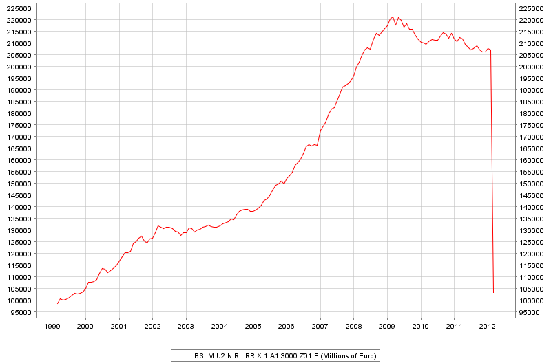
There are other effects. The ECB governing council decided in December to reduce reserve requirements to 1% from 2%  January 18. This “freed up” a lot of collateral banks in the Euro Area needed to pledge to the Eurosystem, thereby providing some relief to the banking system in crisis.

Chart Source: ECB

On 18 January, reserve requirement was €103.33bn as compared to €207.03bn on the previous day.

The Eurosystem And Greek Government Debt

Some bonds of the Greek government mature on March 20. The total principal amount is €14.5bn.

The focus in the financial markets is what will happen to these securities and everyday we read about negotiations with the creditors on “private sector involvement (PSI)”. For the latest see this WSJ article Greece Private-Sector Creditors Meet in Paris.

According to The New York Times DealBook

Brokers estimate that of the 14.5 billion euros of these bonds outstanding, the largest holder is the European Central Bank, which bought these securities in 2010 at a price of around 70 cents in an early, ultimately futile attempt to boost Greece’s failing bond market. The brokers say that 4 billion to 5 billion euros of bonds are owned by hedge funds at an average cost of around 40 cents to 45 cents, with some of the larger positions being held by funds based in the United States that have large London offices.

Let us look at what may happen as far as the Eurosystem is concerned on March 20. Let’s assume that the Eurosystem holds €10bn of the maturing issue – €3bn each by De Nederlandsche Bank and the Bank of Greece and €4bn by the European Central Bank. And that the remaining €4.5bn are held by hedge funds.

Let’s assume that the hedge funds will be paid 15 cents for every € of bond held and are issued new restructured debt securities – i.e., €675m (Plus what about the final coupon payment?)

Question:  Where does Greece get the €10.675bn from?

The ECB is opposed to losses on the Eurosystem’s holdings as per this Bloomberg report from today so it may get a preferred creditor status.

The Eurosystem and the Greek government cannot roll the debt as it will violate the Treaty. So some official creditor or a group of creditors (EFSF?) will have to purchase €10bn+ of bonds from the Greek government before March 20 who will then pay €3bn each to the De Nederlandsche Bank and the Bank of Greece and €4bn the European Central Bank (plus coupons) on March 20 who will then later purchase the bonds from the group of official creditors!

The same holds even if the Eurosystem takes some loss.

Some GIMP Fun With Spain’s Sectoral Balances

… but not fun for the Spanish people.

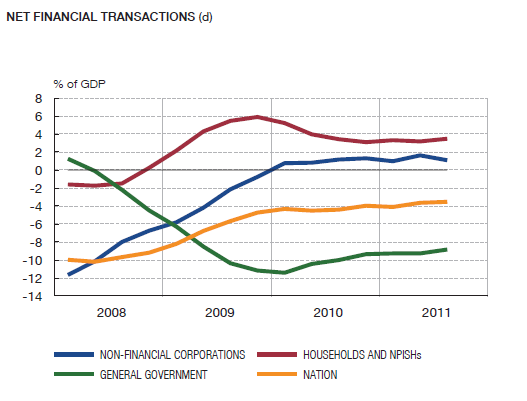
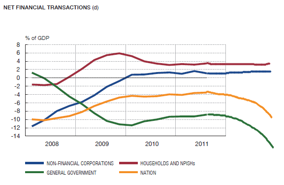
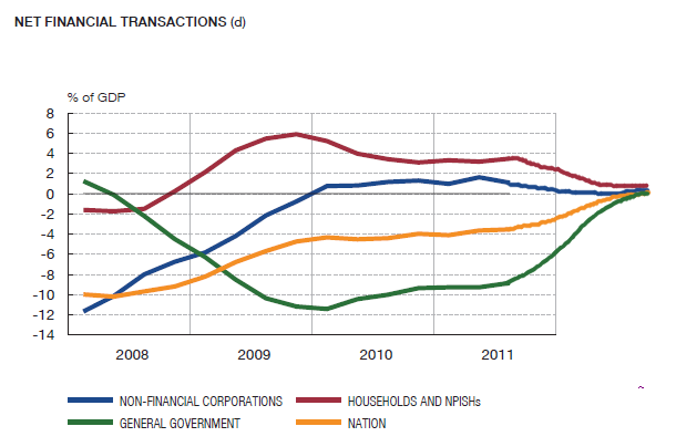
In yesterday’s post Spain’s Sectoral Balances, I briefly discussed the sectoral balances of Spain and its connection with demand, income and output. Here’s the original graph from the Banco de España again with my viewpoints in the previous post.

I learned some GIMP from a friend some time ago and thought I’ll use it for some fun.

I consider two scenarios:

Suppose the Spanish government relaxes its fiscal policy (independent of other Euro Area governments’ policies) or does not tighten it. How do the sectoral balances look? Here’s a likely scenario:

(may not sum to zero because of drawing discrepancies)

The “projection” – not to scale since I had limited availability for space – implies the government deficit keeps rising and this is the result of the rising current account deficit. A higher fiscal stance leads to a slightly higher income and employment but the flip side of this is a rising indebtedness to the rest of the world caused due to the current account deficits. The public sector is incurring almost all the change in net indebtedness – i.e., its contribution to net borrowing from the rest of the world is the highest.

Of course, this process cannot go on forever as a rising indebtedness implies foreigners have to be attracted by hook or crook and interest rate paid on government debt and consequently all private sector debts will also keep rising leading to a deflationary bust at some stage.

Also note, the causality here is a bit opposite of what was described in the previous post! The causalities between the balances of the “three sectors” is complex and not so straightforward. Here a higher fiscal stance leads to a higher income and expenditure and a widening of the current account deficit which in turn widens the budget deficit.

To prevent such possible instabilities – at least their smell of such instabilities – the European leaders have imposed the “fiscal compact” on nations.

What do they aim to achieve? The following “projection” is a possible answer:

The above describes the possible outcome of a tight fiscal stance of the Spanish government. A tight fiscal policy leads to lower income and hence a lower current account deficit – because of lower expenditure on foreign products – but it is achieved via lower output and employment.

The above projections are not based on a specific model for the Spanish economy but some analysis based on familiarity with SFC modelling.

Macroeconomics is not so easy – there are so many constraints – and governments have to strive to achieve the best optimal outcome. “Market forces” do not do that.

The second scenario can also be achieved by a coordinated fiscal expansion by the Euro Area nations. The sectoral balances may behave similar to the second scenario but in the expansionary scenario, output and hence employment is higher. Unfortunately there is no mechanism or institutional means by which fiscal policies are coordinated within the Euro Area (the exception is the recent “fiscal compact” which unfortunately misses the point). Even if there is an agreement on fiscal expansion, there is nothing to make sure that there is a constant management of the whole process – i.e., there are chances of failure.

There are various ideas one sees on proposing a solution to end the Euro crisis but almost none appreciate the real problems. In my opinion, there is no alternative to moving ahead with a European integration and granting more fiscal powers to the European powers – making it a central government – which is involved in fiscal transfers and a mandate to achieve full employment.

Spain’s Sectoral Balances

The Banco de España released its Quarterly Economic Bulletin today and it had an interesting chart on the sectoral balances of the Spanish economy.

With a net indebtedness of €994.5bn – i.e., close to €1 trillion – as compared to the gross domestic product of €1.06tn (2010 figure) Spain has limited choices. Except via the possibility of expanding by another private sector led credit expansion which is highly unlikely, the Spanish economy faces the prospects of low output and demand. Increasing exports is another option but with all Euro Area nations’ governments being forced by a “fiscal compact” to contract, this is unlikely because of low demand in the rest of Europe.

The chart is really interesting as it illustrates some of the many causalities associated with the financial balances identity

NAFA = PSBR + BP

where NAFA is the Net Accumulation of Financial Assets of the domestic private sector, PSBR is the Public Sector Borrowing Requirement or the deficit and BP is the current balance of payments.

When the domestic private sector tries to increase its saving, there is a contraction of demand, income and output (unless exports increase). As a result imports too reduce (because income is lower). The higher propensity to save also leads to an increase in the government’s budget balance.

So in the chart you see a dramatic fall in the current account deficit and a huge increase in the government’s budget deficit. (The term “Nation” is used in the chart because the current balance of payments is the difference between the incomes and expenditures of all domestic sectors of a nation).

The situation is not atypical of recent (post crisis) behaviour of other nations’ sectoral balances but the fall in the external sector balance in this case is striking, though the same could be said for various deficit nations in the Euro Area.

The Banco de España – whose short-term projections are usually accurate – also said today that unemployment will hit 23.4% in 2012!