Yearly Archives: 2016

Discrete Time Or Continuous Time?

There is always some debate by people on how continuous time is better modelling. A James Tobin quote from his Nobel Lecture comes to mind.

Macroeconomic Modeling Strategy: Continuous or Discrete Time

The issues just discussed are related to the modeling of time. The equations introduced above count time in discrete periods of equal finite length. Within any period, each variable assumes one and only one value. In particular, clearing of asset markets determines one set of asset prices per period. From one period to the next asset stocks jump by finite amounts. Therefore the demands and supplies for these jumps affect asset prices and other variables within the period, the more so the greater the length of the period. They will also, of course, influence the solutions in subsequent periods.

The same modeling strategy can be used with continuous time. The specific saving functions, as well as the total saving function, then tell the rate at which savers want to be increasing their stocks of particular assets and of total wealth. They will reflect both the continuous execution of long run saving and portfolio plans and the speeds of adjustment of stocks to deviations from these plans that arise because of surprises, news, and altered circumstances or preferences.

Either representation of time in economic dynamics is an unrealistic abstraction. We know by common observation that some variables, notably prices in organized markets, move virtually continuously. Others remain fixed for periods of varying length. Some decisions by economic agents are reconsidered daily or hourly, while others are reviewed at intervals of a year or longer except when extraordinary events compel revisions. It would be desirable in principle to allow for differences among variables in frequencies of change and even to make those frequencies endogenous. But at present models of such realism seem beyond the power of our analytic tools. Moreover, many statistical data are available only for arbitrary finite periods.

Representation of economies as systems of simultaneous equations always strains credibility. But it takes extraordinary suspension of disbelief to imagine that the economy solves and re-solves such systems every microsecond. Even with modern computers the task of the Walrasian Auctioneer, and of the market participants who provide demand and supply schedules, would be impossible. Economic interdependence is the feature of economic life and we as professional economists seek to understand and explain. Simultaneous equations systems are a convenient representation of interdependence, but it is more persuasive to think of the economic processes that solve them as taking time than as working instantaneously.

In any event, a model of short-run determination of macroeconomic activity must be regarded as referring to a slice of time, whether thick or paper thin, and as embedded in a dynamic process in which flows alter stocks, which in turn condition subsequent flows.

Subscripting Helps!

The accounting identities equating aggregate expenditures to production and of both to incomes at market prices are inescapable, no matter which variety of Keynesian or classical economics you espouse. I tell students that respect for identities is the first piece of wisdom that distinguishes economists from others who expiate on economics. The second? … Identities say nothing about causation.

– James Tobin, 1997, p. 300, ‘Comment’, in B.D. Bernheim and J.B. Shoven (eds), National Saving and Economic Performance, Chicago: University of Chicago Press.

This is a continuation of my post Stock-Flow Inconsistent? which was a reply to Jason Smith’s blog post More like stock-flow inconsistent on his blog Information Transfer Economics. If you had checked my post before around noon UTC yesterday, you might want to check the updated version.

Jason Smith also has updated his post and proposes a new equation:

ΔH = Γ·(G – T)

(incorrect equation)

Now, that’s quite wrong because it violates rules of accounting.

Morever, Jason Smith insists that it is a behavioral equation.

A lot of clarity can be achieved if one uses subscripts, so that things are clearer.

So we have two equations:

ΔH = GT

dH/dt = GT

Although these two are related, they are not exactly the same: the former is in a difference equation form and the latter in the differential equation form. The in the former has no time dimensions and the in the latter has time dimension equal to –1. The in the former is total expenditure in a period, the in the latter is a rate. 

Since stock-flow consistent models are written typically in difference equations, rather than differential equations, let us avoid subscripts for difference equations for the former and use it for latter.

So it is better to write the equations as:

ΔH = G – T

dHcontinuous/dt = Gcontinuous – Tcontinuous

Each time step in the formalism of difference equations is Δt and hence

G = Gcontinuous ·Δt

T = Tcontinuous ·Δt

Hcontinuous = H

So,

ΔHt = Gcontinuous – Tcontinuous

(approximately)

Or,

ΔH/ Δt = Gt – Tt

Or,

ΔH = G – T

So instead of reaching the correct equation which is:

ΔH= Δt · (Gcontinuous – Tcontinuous)

Jason reaches the equation:

ΔH = Γ·(G – T)

(incorrect equation)

But

ΔH = G – T

as it is an accounting identity in the model!

Stock-Flow Inconsistent?

The first rule of Post-Keynesian Economics is: You do not talk make accounting mistakes. The second rule of Post-Keynesian Economics is: You do not talk make accounting mistakes.

– Anonymous.

Jason Smith—who is a physicist—but writes a blog in Macroeconomics, wonders how equations in the simplest stock-flow consistent model given in the textbook Monetary Economics written by Wynne Godley and Marc Lavoie make any sense from a dimensional analysis viewpoint.

He says he

seem[s] to have found a major flaw.

He sees the equation:

ΔH = GT

and wonders where the time dimensions are. For, H is the stock of money and hence has no time dimension, whereas the right hand side has flows and has time dimensions of inverse of time. For example if the US government spends $4 tn in one year, is $4 tn/year.

In continuous time, the above equation is:

dH/dt = GT

So how are these two equations the same?

Perhaps, Jason is not familiar with difference equations. He instead seems to prefer:

τ·ΔH = GT

Well that’s just wrong if τ is anything different from 1, as a matter of accounting.

Now moving on to time scales, it is true that in difference equations some time scale is implicit. But it doesn’t mean the methodology itself is wrong. Many physicists for example set all constants to 1 and then talk of numbers which are dimensionless.

So if a relativist sets “c=1”, i.e, the speed of light to 1, all velocities are in relation to the speed of light. So if somebody says the speed is 0.004, he/she means the speed is 0.004 times the speed of light.

But Jason Smith says:

Where does this time scale come from over which the adjustment happens? There is some decay constant (half life). It’s never specified (more on scales here and here). If you think this unspecified time scale doesn’t matter, then we can take Δtlp and the adjustment happens instantaneously. Every model would achieve its steady state in the Planck time.

That’s not true. String theorists for example set the parameter α’ = 1. But nobody ever claims that macroscopic adjustments happen at Planckian length scales or time scales.

Coming back to economics, there’s nothing wrong in

ΔH = GT

There’s an implicit time scale yes, such as a day, or a month, or a year, or even an infinitesimal. But parameters change accordingly. So in G&L models we have the consumption function

 C = α1 ·YD + α2 ·W

where is household consumption, YD, the disposable income and W, the household wealth.

Let’s say I start with a time period of 1 year for simplicity. αmight be 0.4. But if I choose a time period of 1 quarter, αwill correspondingly change to 0.1. In English: if households consume of 4/10th  of their wealth in one year, they consume in 1/10th one quarter.

So if we were to model using a time scale of a quarter instead of a year, α2 will change accordingly.

But the equation

ΔH = GT

won’t change because it is an accounting identity!

It’s the difference equation version of the differential equation:

dH/dt = GT

Physicists can pontificate on economic matters. I myself know string theory well. But boy, they shouldn’t make mathematical errors and embarrass themselves!

In other words, accounting identities can be written as accounting identities in difference equations. What changes is values of parameters when one chooses a time scale for difference equations.

Wynne Godley’s model is touched by genius. In fact according to one of the reviewers of Monetary Economics, Lance Taylor says that it is out of choice that Wynne Godley chose a difference equation framework. They can be changed to differential equations and we’ll obtain the same underlying dynamics.

Here’s Lance Taylor in A foxy hedgehog: Wynne Godley and macroeconomic modelling

Godley has always preferred to work in discrete time, responding to the way the data are presented.

Question: is the equation ΔH = Gconsistent with dimensional analysis?

Answer: Yes. H is the stock of money at the end of previous period. Δis the change in stock of money in a period. and are the government expenditure and tax revenues in that period. So H, ΔH, G and T have no times dimensions in difference equations. All are in the unit of account. Such as $10tn, $400bn, $4 tn, $3.6tn. Time dynamics is captured by model parameters.

In G&L’s book Monetary Economics, in Appendix 3 of Chapter 3, there’s a mean-lag theorem, which tells you the mean lag between two equilibrium (defined as a state where stock/flow ratios have stabilized):

it is:

[(1 − α1)/α2 ]· [(1 – θ)/θ]

where θ is the tax rate.

So, in the model, assuming a value of 0.6 for α1, 0.4 for α2, and 0.2 for θ we have the mean-lag equal to 4.

Let’s assume that time period is yearly. This means the mean lag is 4 years.

If instead, we were to use quarterly time periods, α2 would be 0.1 and the mean lag evaluates to 16, i.e., sixteen quarters, which is 4 years, same as before.

So there is really no inconsistency in stock-flow consistent models.

tl;dr summary: In difference equations, there’s nothing wrong with equations such as ΔH = GT. It is an accounting identity. By a choice of a time scale, one implicity chooses a time scale for parameter values. What’s wrong? Jason Smith would obtain the same results as the simplest Godley/Lavoie model if he were to work in continuous time and write equations such as dH/dt = GT. I will leave it to him as an exercise!

Occult Or Investment Banky?

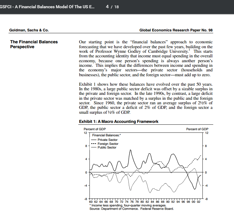
Noah Smith has a blog post calling heteredox economics occult. Rather than write a long post which nobody will read, let me point out that Goldman Sachs’ chief economist Jan Hatzius uses Wynne Godley’s model. He frequently cites Wynne Godley (and only him!) for his model as well.

Noah Smith is a fan of investment banks and Goldman Sachs being the top firm should make him realize the importance of heterodox modelling.

Not only does heterodox economics have a framework, it is used by the top investment banking firm!

Here’s are two screen snips of GS’ paper written by their chief economist Jan Hatzius and describing their model in detail.

Jan Hatzius Paper Using Wynne Godley's Work

Jan Hatzius’ paper dated September 18, 2003

Jan Hatzius Paper Using Wynne Godley's Work - 2

Jan Hatzius acknowledging Wynne Godley for his model of the US economy 

Heterodox Blogger On Neochartalism

The trouble with Neochartalism (and called “Modern Monetary Theory” by the Neochartalists) is that what is correct is not original and what is original is not correct.

A popular heterodox blogger writing under the pen name “Lord Keynes” and blogging at Social Democracy For The 21st Century has written a post Limits Of MMT

It’s good to see the blogger point that the main trouble with Neochartalism is the balance of payments constraint. He/she has said this in the past in posts while promoting it, so it’s good to see a special post for this. I don’t agree with many things with “Lord Keynes” but given the blog’s popularity, I think it’s a good thing to have happened.

There is one thing I would have liked to see differently. It is sometimes said that Neochartalism works for advanced/rich nations and not for poor nations. But this gives too much importance to Neochartalism. This is because the rise and fall of nations itself depends on competitiveness in international markets. Saying “MMT works for advanced nations” makes it look as if the success and failure of nations is to be explained elsewhere. It’s still true of course that advanced nations can expand domestic demand by fiscal expansion but they also have to look after the being being of firms selling products in international markets, to stay competitive and not lose edge. Similarly as the blogger Lord Keynes says, “What is needed for much of the Third World is heterodox development economics, not MMT.”

More generally a concerted action is needed by world political leaders in which fiscal policies are coordinated with a set of consistent balance of payments targets.

Neochartalism has confused people more than they were confused earlier. It has to be debunked.

The World Balance Of Payments Constraint: Nicholas Kaldor Explaining The Way The World Works

Thirlwall’s Law is counter-intuitive and comes across as shocking. It says that the growth of a nation’s economy is directly proportional to the rate of exports and inversely related to the income elasticity of imports.

The reason it comes as shocking and difficult to believe is that our planet, with all inhabitants and institutions considered resident cannot export (unless there are non-residents such as aliens), but the world still grows.

Now there are several pitfalls in this argument. First, Thirlwall’s law doesn’t fail because the expression for growth rate is indeterminate. Rate of exports is indeterminate and the income elasticity of imports is indeterminate.

So we have

growth = inderminate/indeterminate

Second, the world does not have a central government. So the world as a whole is not comparable to a closed economy with a government.

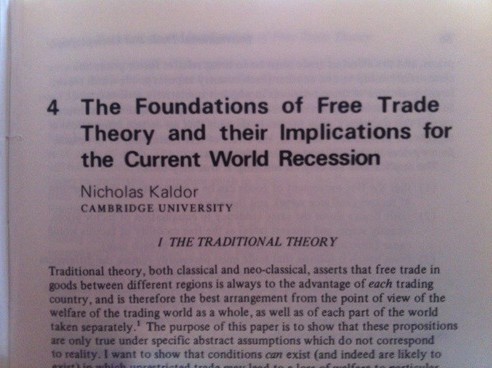
There is a way in which the world as a whole is balance-of-payments constrained. The argument is by Nicholas Kaldor. In his 1980 article Foundations And Implications Of Free Trade Theory, written in Unemployment In Western Countries – Proceedings Of A Conference Held By The International Economics Association At Bischenberg, France, Kaldor makes the argument for the world balance-of-payments constraint.

Nicholas Kaldor On Free Trade

Nicholas Kaldor on free trade

In a recent article on the ‘Causes of Growth and Recession in World Trade’,1 T. F. Cripps has demonstrated that a country is not ‘balance of payments constrained’ if its full employment imports, M*, are less that its import capacity M̅ (as determined by its earning from exports). Such a country is free to choose the level of domestic demand which it considers optimal for its own circumstances,2 whereas the other countries from whom M* > M̅, must, under conditions of free trade, reduce their output and employment below the full employment level, and import only what they can afford to finance. He then shows that the sum of imports of the ‘unconstrained’ countries determine the attainable level of production and employment of the ‘constrained’ countries, and the remedy for this situation requires measures that increase the level of ‘full-employment’ imports or else reduce the export share of the ‘unconstrained countries’. The ‘rules of the game’ which would be capable of securing growth and stability in international trade, and of restoring the production of the ‘constrained’ countries to full employment levels, may require discriminatory measure of import control, of the type envisaged in the famous ‘scarce currency clause’ of the Bretton Woods agreement.

In the absence of such measures all countries may suffer a slower rate of growth and a lower level of output and employment, and not only the group of countries whose economic activity is ‘balance-of-payments constrained’. This is because the ‘surplus’ countries’ own exports will be lower with the shrinkage of world trade, and they may not offset this (or not adequately) by domestic reflationary measures so that their imports will also be lower. Provided that the import regulations introduced relate to import propensities (i.e. to the relation of imports to domestic output) and not to the absolute level of imports as such, the very fact that such measures will raise the trade, production and employment of the ‘constrained’ countries will mean that the volume of exports and domestic income of the ‘unconstrained’ countries will also be greater, despite the downward change in their share of world exports.3

Footnotes:

1Cambridge Economic Policy Review (March 1978), pp, 37-43.

2Owing to the widespread view according to which a given increase in effective demand is more ‘inflationary’ in its consequences if brought about by budgetary measure than if it is the result of additional investment or exports (irrespective of any limitations of import capacity) the inequality or potential inequality in its payments balance may cause a surplus country to regard a lower level of domestic demand as ‘optimal’ in the first case than in the second case.

3In other words, if countries whose ‘full employment’ balance of payments shows a surplus because M* < α W (where M* is the level of full employment imports, α is the share of a particular country’s exports of in world trade W) after a reduction of α to α̂ (α̂ < α) through the imposition of discriminatory measures, the country will still be better off if α̂ W* > α W where W* is the volume of world trade generated under full employment conditions.

[boldening mine]

What Kaldor is saying that because of balance of payments constraint of economies, the world as a whole has a slower growth because surplus nations do not expand domestic demand to the level needed. He is also saying that import controls raise imports rather than reduce them (this because of higher national income) and the exporters’ exports will also increase (even though their share is reducing.).

So the world as an built-in deflationary bias in the way it works.

Limits To Growth, Part 3

[For previous discussions, see my posts Limits To Growth? and The Full Employment Assumption]

Brian Romanchuk has written a post as a response to my post Limits To Growth? referred above. In that his tone seems to be that the U.S. does not face an external constraint fundamentally, and that trade acts as a drag only because politicians have an impression that there exists a constraint.

To hold that claim Brian should to able to defend the dynamics which is likely if that were the case: the U.S. public debt and the net international investment positions deteriorate without limit (relative to gdp). Not sure at the moment if he thinks that debt/gdp ratios can grow without any limit.

That is the financial aspect of his argument. From the trade perspective, Brian says:

In any event, the U.S. could get away with strong GDP growth without causing external difficulties right now. There is plenty of spare global manufacturing capacity, so rapid U.S. growth would be accommodated by exporters. After awhile, there would be a self-reinforcing global growth spurt, which will reduce the pressure on the U.S. trade balance.

There are two things. One is capacity constraint and the other competitiveness.  Both I and Brian agree there is no need to worry about the former. (Unlike neoclassical economists who are worried about the former!). It is about the latter where the debate is. This is in addition to the financial aspect mentioned in the previous paragraph.

The U.S. having plenty of spare manufacturing capacity has little impact on competitiveness. At a micro level, one can think of a firm with lots of idle resources but the sales team not being able to win projects for the firm. So two things—capacity and competitiveness—need to be studied separately. If the rest of the world does not expand, there is not much U.S. firms can do. If they produce more stuff, it will just be left as additional inventories forcing a clearing sale in domestic markets at the year end. So presence of spare capacity cannot make U.S. exports grow if domestic demand rises, either due to rise in private expenditure or via fiscal policy. In addition, there’s no self-reinforcing global growth because exports won’t take off to begin with.

To be more technical, there is one way in which U.S. exports may rise. If production rises, then via the Kaldor-Verdoorn process, U.S. productivity will also rise and this affects pricing of products and U.S. exporters may get some price advantage.

So rise in production can lead to a rise in competitiveness.

But this effect is quite negligible in the short run because competitiveness is both about non-price competitiveness and price competitiveness. 

There is an additional effect. U.S. production rising means rise in national income and rise in imports. This implies a rise in global output and demand and helping U.S. exports. Again, this effect is small and doesn’t prevent a deterioration of balance of payments and international investment position. So U.S. production rising helps exporters a bit but not much.

What the world needs is a coordinated policy to raise output by fiscal policy and putting limits on balance of payments imbalances.

Whoever becomes President of the United States has to not only take care of domestic policies but also act as a leader in world wide policy.

All this is about the future. But it’s not that the U.S. balance of payments hasn’t mattered in the past. Because of imbalances in trade, the U.S. fiscal policy could not save the U.S. i.e., could not bring the economy back into full employment quickly. It has taken about 9 years and there is still not full employment. So much has been lost. The critical imbalance in U.S. trade is the numero uno reason for the lack of a quick recovery. It could be said that the U.S. could have expanded fiscal policy and that is quite true but it would have put the U.S. debts on unsustainable path.

Digression

It is sometimes said, such as by a commenter in Brian’s blog that “balances balance”, so there is no need to worry about them. There is no imbalance as per an economist. This is a dubious argument. Surely the private sector can be in deficit for long and it is matched by items in the financial account of the system of national accounts. But surely private sector deficits for long is unsustainable as agreed by everyone around here. So “balances balance” is no argument.

The Full Employment Assumption

Before I begin, Brian Romanchuk has written a reply to my previous post. Highly likely you have seen it, but if you haven’t check it out. I will reply soon but for now I want to tackle neoclassicals economists’ dubious claims.

The background for readers not having seen recent debates is that Paul Krugman has launched a vicious attack claiming that it is not possible for the U.S. economy to grow at 5.3%. His analysis is just some random averaging of numbers more than anything else. In my argument, it doesn’t matter if it is Bernie Sanders or someone. The question is just about possibilities. The question is: is 5.3% possible in the next four US presidential years?

First, 5.3% over four years is about 23%.

The United States doesn’t have full employment. A lot of people are working part time and many others are discouraged from work. So cannot the U.S. government boost domestic demand and raise real GDP by 23% in four years?

Of course, it can do it.

But the debate has been hijacked by debating purely about productivity. Here’s Noah Smith for example:

click to view the tweet on Twitter

So neoclassical economists are making it look as if it is only a matter of rise in productivity.

(Update: Smith has written an article for Bloomberg here)

I am going to argue that productivity is really a sideshow.

Why does productivity matter? If there is full employment and no additions to the labour force, production can only rise if productivity rise. This is purely a matter of definitions and not a causal statement. In fact, the causality is from production to productivity and not the other way round. But if there isn’t full employment, production can rise even if there is no rise in productivity. It’s just about more people who were not employed before, producing more stuff. In addition a lot are also joining the labour force for the first time. So production can rise without productivity rising.

Now with high unemployment and people working part time and people discouraged from looking for work, it is entirely possible that almost the whole of 23% is purely attributed to this.

Think Okun’s Law.

So productivity rises is really a sideshow here. But it’s good if it rises. But it’s sad that the debate is centred around productivity rises.

In summary 23% can be reached by

  1. Rise in production attributable to no rise in productivity
  2. Rise in productivity. (Caused by the rise in production itself).

The debate is centred around the point 2. This is not surprising. Neoclassical models are built assuming full employment, so an economist is simply trained to think of point 2 and not think about point 1 at all. As Joan Robinson would say:

Before ever he [a student] does ask, he has become a professor, and so sloppy habits of thought are handed on from one generation to the next.

Limits To Growth?

There has been a debate led by vicious attack by Paul Krugman that Bernie Sanders’ plans cannot achieve growth of 5.3%. And there have been replies by others.

Coming from a third-world country and seeing an annual growth rate of about 8% in the 10 years of the rule of the UPA government (mid 2004-mid 2014), —meaning real GDP more than doubling in 10 years — despite a global financial crisis and economic slowdown, it appears comical to me that Paul Krugman claiming such a thing is not possible for the United States.

I am a bit unsympathetic to those who quote historical data to try to sneak in an argument that 5.3% is possible. It sounds too apologetic.

If the U.S. fiscal policy was run with a restrictive bias since a long time, there is obviously a huge deflationary bias imparted by policy. So you cannot use that data to either argue one way or the other. The ones using data to try to show it’s possible are playing into the hands of economists such as Paul Krugman whose writing appears nothing but a support for Hillary Clinton.

For a closed economy, the only constraint to growth is the capacity to produce. The United States’ economy suffers no such constraint. At full employment, growth is constrained by rises in productivity and addition to the working population. But productivity itself is endogenous to production because of learning by doing. In addition, rises in incomes motivate people to work harder.

So imagine an economy in which the government’s fiscal stance is held constant for 10 years – i.e., the government expenditure and the tax rates are held constant. Output might fluctuate and even grow but finally the deflationary bias in fiscal policy will drag growth. But you cannot average out 10 years of economic data of hardly any growth to argue out that the economy cannot grow for the next n years.

But things are not easy. What surprises me is that in none of these discussions from either side, is there any discussion of the U.S. balance of payments. The U.S. does not have exports of just a couple of hundred billions and a GDP of some $16 tn. It has exports of about $2.5 tn and GDP of about $16 tn, meaning the GDP is a few multiple of exports. The United States is a net debtor to the rest of the world. So a rapid rise in growth by any means will come at the expense of terribly deteriorating balance of payments which cannot last long.

Of course the above doesn’t mean that things are as pessimistic. It depends on what is going on in the rest of the world and the United States being the economic center of world activity can convince others to boost their economies and there is no reason to assume that it cannot. if there is rapid growth in other economies, the U.S. balance of payments is not something to worry about.

The importance of balance of payments is seriously missing in all discussions. Use of historical data is so wrong here.

tl;dr summary: supply constraints cannot put a limit of some 5% on U.S. growth. It depends on policy makers’ decisions worldwide.

February 11

I normally don’t like The Economist as it promotes free trade between nations and historically that was the reason it started publishing and became popular. I however liked its description of the detection of gravitational waves:

TWO black holes circle one another. Both are about 100km across. One contains 36 times as much mass as the sun; the other, 29. They are locked in an orbital dance, a kilometre or so apart, that is accelerating rapidly to within a whisker of the speed of light. Their event horizons—the spheres defining their points-of-no-return—touch. There is a violent wobble as, for an instant, quintillions upon quintillions of kilograms redistribute themselves. Then there is calm. In under a second, a larger black hole has been born.

And then, 1.3 billion years later, in September 2015, on a small planet orbiting an unregarded yellow sun, at facilities known to the planet’s inhabitants as the Advanced Laser Interferometer Gravitational-wave Observatory (LIGO), the faintest slice of those waves was caught. That slice, called GW150914 by LIGO’s masters and announced to the world on February 11th, is the first gravitational wave to be detected directly by human scientists. It is a triumph that has been a century in the making, opening a new window onto the universe and giving researchers a means to peer at hitherto inaccessible happenings, perhaps as far back in time as the Big Bang.