Author Archives: V. Ramanan

Interest Rates And Investment

There is a new interesting Federal Reserve paper The insensitivity of investment to interest rates: Evidence from a survey of CFOs.

Abstract:

A fundamental tenet of investment theory and the traditional theory of monetary policy transmission is that investment expenditures by businesses are negatively affected by interest rates. Yet, a large body of empirical research offer mixed evidence, at best, for a substantial interest-rate effect on investment. In this paper, we examine the sensitivity of investment plans to interest rates using a set of special questions asked of CFOs in the Global Business Outlook Survey conducted in the third quarter of 2012. Among the more than 500 responses to the special questions, we find that most firms claim to be quite insensitive to decreases in interest rates, and only mildly more responsive to interest rate increases. Most CFOs cited ample cash or the low level of interest rates, as explanations for their own insensitivity. We also find that sensitivity to interest rate changes tends to be lower among firms that do not report being concerned about working capital management as well as those that do not expect to borrow over the coming year. Perhaps more surprisingly, we find that investment is also less interest sensitive among firms expecting greater revenue growth. These findings seem to be corroborated by a cursory meta-analysis of average hurdle rates drawn from firm-level surveys at different times over the past 30 years, which exhibit no apparent relation to market interest rates.

The survey makes sense on a cursory look and lot of economists – especially Post-Keynesians assume away the interest sensitivity of interest rates on business investment in models many times. This is because demand for their goods and services is far more important than interest payments.

There are many complications however. Inventory building can have sensitivities to interest rates – although this may not be too significant. I am not sure the same can be said for house purchases. People’s knowledge of movements of mortgage rates can sometimes be surprising. If interest rates are dropped, households can purchase more houses on credit and this leads to a higher output and higher national income and more demand for firms’ products and services inducing more business investment – a multiplier effect. So indirectly interest rates can be said to have an effect on business investment. A resultant stock market rise – if there is one – can lead to wealth effects i.e., rise in output caused by rise in consumption due to capital gains and rise in household wealth.

One can think of international effects as well. If other central banks do not change interest rates, the domestic currency can depreciate against foreign currencies and this may slightly improve price-competitiveness of firms compared to foreign firms and improve exports and lead to some amount of imports substitution. This will have its own multiplier effect.

Of course like other channels mentioned above, this is not guaranteed to work and to the extent needed. A drop in the short term interest rate by the central bank can induce portfolio investment from abroad into equities and the exchange rate may not fall and instead rise. Also if households incomes have dropped due to a recent recession, they may not buy homes just because interest rates have dropped.

What about the reverse? A rise in interest rates – in addition to a reduced demand for house purchases – can lead to a higher interest burden of households on existing loans for house purchases, reduce domestic demand due to a drop in consumption and cause a fall in firms’ investment.

This post of course just touches these things and isn’t a claim to be anything like a full analysis. Models can be helpful in bringing these things more clearly. But models themselves have limitations so one needs a mix of empirical analysis to study such things.

Even empirical studies may be difficult.  Nicholas Kaldor’s in his 1958 article Monetary Policy, Economic Stability And Growth (republished in Collected Essays, Vol. 3, page 133) points out:

It must be remembered that in times of full employment, or even of approximately full employment, the capacity of the investment goods industries may exert a far more important limitation on the level of capital expenditure than the cost of borrowing or the availability of particular forms of finance. Thus the rate of building and constructional activity may be confined by the availability of building and constructional labour; expenditure on plant and equipment may be limited by lengthening delivery periods on new contracts. In such situations, the range of projects whose execution would be influenced by changes in the cost of borrowing or in the availability of loans might be unusually narrow …

So if we have some empirical data, how do we decide whether the slowdown of output in whichever period in the data the output slowed down was caused due to an increase in short term interest rate by the central bank or because of capacity constraints? The answer in my opinion is more empirical research and more model building.

It is also worth mentioning that despite so many complications, the economics profession pretends that fiscal policy is somewhat less important and ignores it as compared to monetary policy. Things have changed a little during after the crisis but one never knows when they take a U-turn on such issues.
Augusto Graziani And The Theory Of The Monetary Circuit

One of Augusto Graziani’s best papers was The Theory Of The Monetary Circuit, Économies et Sociétés, 24 (6) (June), pp. 7–36. The paper is available at the UMKC course site here.

One description of money is looking at payments as triangular transactions. Graziani says that for money to exist, three conditions have to be met:

  1. since money cannot be a commodity, it can only be a token money;
  2. the use of money must give rise to an immediate and final payment and not a simple commitment to make a payment in the future; and
  3. the use of money must be so regulated as to give no privilege of seignoriage to any agent

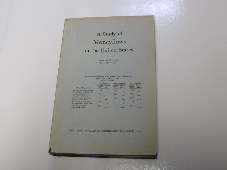
The phrase “money circuit” was actually first used by Morris Copeland – the discover of flow of funds in his book A Study of Moneyflows in the United States

A Study Of Moneyflows In The United States - Morris Copeland

(image credit: Xerxes Books, from whom I obtained the copy)

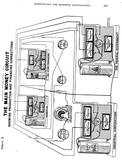
In his book, he actually draws a diagram of a circuit – on the inside covers and on page 245:

The Main Money Circuit

The circuitists’ motivation for using the phrase “circuit” was a circular flow starting with credit but Copeland was in total opposition of the usage of the phrase “hyrdraulic/s” and the misleading notions that this latter phrase conveys about money. Hence he proposed the phrase money circuit. Check his book on why this is so for details. I will at some point write about Copeland’s arguments.

Augusto Graziani, R.I.P.

Augusto Graziani has died.

One of Graziani’s main themes runs as follows. In order to finance production, the entrepreneur must obtain the funds necessary to pay his workforce in advance of sales taking place. Starting from scratch, he must borrow from banks, at the beginning of each production cycle, the sum which is needed in order to pay wages, creating a debt for the entrepreneur and, thereby, an equivalent amount of credit money, which sits initially in the hands of the labour force. Production now takes place and the produced good is sold at a price which enables the debt to be repaid inclusive of interest, while hopefully generating a surplus – that is, a profit – for the entrepreneur. When the debt is repaid, the money originally created is extinguished. An entire monetary circuit is now complete.

This account of the monetary circuit has a number of extremely important and distinctive features. It emphasises, in particular, that a) there is a gap in (historical) time between production and sales which generates a systemic need for finance; b) bank money is endogenously determined by the flow of credit and c) total real income must be considered to be divided into three parts – that received by entrepreneurs, that received by labour and that received by banks. We have already travelled an infinite distance from the (yes, silly) neo-classical world where production is (must be) instantaneous, where money must be exogenous and fixed and has no counterpart liability, and where the distribution of income is determined by the marginal products of labour and capital – a construction which depends entirely on the assumption that all firms sit perennially on a single aggregate neoclassical production function frontier.

− Wynne Godley, Weaving Cloth From Graziani’s Thread in Money, Credit And The Role Of The State: Essays In Honour Of Augusto Graziani

Ben Bernanke On Effects Of Federal Reserve LSAP

In a speech at the Annual Meeting of the American Economic Association, Philadelphia, Pennsylvania, Ben Bernanke defended the large-scale asset purchase program of the Federal Reserve (“QE”).

The text is available here and the video is here

Bernanke’s argument is that fiscal policy was tight but yet the U.S. had an economic recovery and unconventional monetary policy helped.

First he talks of headwinds:

Have these unconventional tools been effective? Skeptics have pointed out that the pace of recovery has been disappointingly slow, with inflation-adjusted GDP growth averaging only slightly higher than a 2 percent annual rate over the past few years and inflation below the Committee’s 2 percent longer-term target. However, as I will discuss, the recovery has faced powerful headwinds, suggesting that economic growth might well have been considerably weaker, or even negative, without substantial monetary policy support.

and then identifies tight fiscal policy by both the federal government and state and local governments as one of the headwinds.

I have discussed the factors that have held back the recovery, not only to better understand the recent past but also to think about the economy’s prospects. The encouraging news is that the headwinds I have mentioned may now be abating. Near-term fiscal policy at the federal level remains restrictive, but the degree of restraint on economic growth seems likely to lessen somewhat in 2014 and even more so in 2015; meanwhile, the budgetary situations of state and local governments have improved, reducing the need for further sharp cuts …

It is not easy to see if this is true but it is true that fiscal policy had been tight and Bernanke’s argument is interesting for further analysis.

Happy New Year 2014

Here’s wishing the readers a happy new year. May you (and I) have a prosperous year ahead and learn more about the shell game of economists!

Good time to talk briefly about time.

Joan Robinson was perhaps the best critic of neoclassical economics and she did this by attacking the very basic concepts of mainstream theory. In her essay Time In Economic Theory (1980, Ch 7 in What Are The Questions?: And Other Essays), page 87 in Section 1: ‘Logical Time’ she says:

In a properly specified stationary state, there is no distinction between any one day and any other. On a properly specified growth path, such as a von Neumann ray, exhibiting a particular pace of expansion of employment and of a specified stock of means of production, there is no movement forward and upward or backward and downward, except the movement of the reader’s eye along the curve.

Unfortunately, the great majority of models in the textbooks are not properly specified. Take, for instance, the familiar Marshallian cross of supply and demand curves showing an equilibrium point in the middle. At a price above the equilibrium level, offer exceeds demand, and below, demand exceeds offer.

Now we are told, if price at any moment is not at the equilibrium level, it will tend toward it. This means that historical events are introduced into a timeless picture. As Professor Samuelson kindly explained to me, ‘When a mathematician says “y rises as  x falls”, he is implying nothing about temporal sequences or anything different from “When x is low, y is high”.’ 

To move implies a temporal sequence. To fill in the story of a movement towards equilibrium, a complicated dynamic process must be specified and to specify a process that will actually reach equilibrium is by no means a simple matter.

[emphasis added]

A footnote refers to page 138 of the book – another essay quoting Samuelson:

[Samuelson]: I do not think that the real stumbling block has been the failure of a literary writer to understand that when a mathematician says, ‘rises as falls’, he is implying nothing about temporal sequences or anything different from ‘when is low, is high’.

Robinson’s response is:

My dear sir! That is my point. I really cannot allow you to get away with that.

Unfortunately, economists keep getting away from this.

Joan Robinson - What Are The Questions And Other Essays Back CoverBack cover of What Are The Questions? …  And Other Essays

Description Of Cryptocurrencies Using SNA

In India – at least a while ago – they were many tickers trading on the stock exchanges with no income and in some cases with no office whatsoever!

Why would anyone incorporate such a thing? For two – illegal – reasons: first the IPO of the company gets the money in – which makes the owners rich – and the second way is to manipulate the price of the stock to fool more investors. The owners would trade among themselves and fool trend followers to buy the stock.

Cryptocurrencies are like that – with the difference being that they are equity liabilities of unincorporated and unregistered enterprises trading in unregulated markets. The deceit lies in marketing them as some sort of currency and inducing people to trade in them as if it were some currency.

If that is the case, what is the national accounts description (like the 2008 SNA) of such a thing? First, there is no incorporation so we have to treat them as quasi-corporations as national accountants do.

Sec 4.42 of the 2008 SNA has a description of quasi-corporations. That is for general economic activity but here I use the concept to describe cryptocurrencies. The difference here is that unlike the quasi-corporations, the cryptocurrency quasi-corp has no income!

The other reason for thinking of a quasi-corporation is that one usually sees money as a liability of an institution, so we need to think of cryptocurrencies as a liability of some economic unit.

So how does the balance sheet of this cryptocurrency quasi-corp look like at various stages?

Let us say that the cryptocurrency quasi-corporation raises $100mn at the “IPO”:

Assets

Liabilities and Net Worth

Bank Deposits = +$100mn

Equities Issued = +$100mn
Net Worth = $0

Note: Here the symbol $ is for the United States dollar and not for any cryptocurrency such as the bitcoin.

Now, the owners of the cryptocurrency quasi-corporation make a “withdrawal of equity”. That is, whatever money is received in ordinary currency is transferred to the owner’s personal account. After this, the balance sheet of the quasi-corporation looks like:

Assets

Liabilities and Net Worth

Bank Deposits = $0

Equities Issued = +$100mn
Net Worth = −$100mn

which has a counterpart that the owners’ net worth rises by $100mn (as a result of the transfer of payment received in dollars to the owners’ account).

Once the “cryptocurrency” starts trading in unregulated markets, the price of a unit rises or falls, so let’s say it rises 10 times the IPO price. At the time,

Assets

Liabilities and Net Worth

Bank Deposits = $0

Equities Issued = +$1bn
Net Worth = −$1bn

Of course, there is nothing wrong with the net worth of a corporation going negative – as may sometimes happen in times when there is a stock market boom, even for the corporate sector of a nation as a whole.

In this case however, this cryptocurrency quasi-corporation has no income whatsoever. In fact, it is using your services and hence making a loss which is covered by issuing more equities!

There is a concept of mining in cryptocurrency which is the most interesting part.

So suppose users “mine” cryptocurrency worth $100mn by providing services to the quasi-corporation, the balance sheet of the quasi-corporation will look like (assuming the price of the cryptocurrency hasn’t changed):

Assets

Liabilities and Net Worth

Bank Deposits = $0

Equities Issued = +$1.1bn
Net Worth = −$1.1bn

In the language of flows, the cryptocurrency quasi-corporation has:
an operating surplus of minus $100mn,
a balance of primary income of minus $100mn,
entrepreneurial income of minus $100mn,
disposable income of minus $100mn, and,
saving (undistributed profits) of minus $100mn.

This has a counterpart in the financial account as a net borrowing of $100mn by issuance of equities worth $100mn.

(For the above refer to the tables in Annex 2 – The Sequence of Accounts of the SNA).

The ultimate user of this intermediate consumption is another firm but the trick here is that its costs are reduced because of the issuance of cryptocurrencies for which it is not liable at all.

In the case where you own some cryptocurrency and pay for some pizza using it, it is a transaction between you and the pizza maker and shouldn’t affect the accounts of the quasi-corporation except the change in the name of ownership of the cryptocurrency – like a transaction using bank deposits. Here it is more like buying a pizza using Apple stocks with Apple Inc. acting as the settlement agent.

Of course, I repeat – currencies are not like equities but in this case, cryptocurrencies have been marketed as currencies whereas they are more like stock market equities but traded in unregulated markets.

The cryptocurrencies are thus a more sophisticated version of stocks of companies trading in markets with no income and no office.

Happy Holidays

Here’s wishing the readers of this blog a happy holiday break.

Happy Holidays

 via hallmark.com

I can never repeat this often enough – always remember:

The purpose of studying economics is not to acquire a set of ready-made answers to economic questions, but to learn how to avoid being deceived by economists.

– Joan Robinson, 1955, “Marx, Marshall And Keynes”, Occasional Paper No. 9, Delhi School of Economics. Also in Collected Economic Papers, Volume Two, 1960.

Peace!

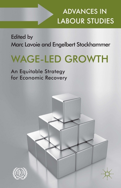
Good Reference On Wage-Led Growth

An excellent discussion on wage-led economic growth is a paper by Marc Lavoie and Engelbert Stockhammer titled Wage-led Growth: Concept, Theories And Policies which appears in the recently released book Wage-Led Growth: An Equitable Strategy For Economic Recovery (Palgrave Macmillan book page)

Wage-Led GrowthFrom the article:

… The advocacy of a wage-led economic strategy has a long history. It has been articulated in reformist visions within the labour movement and was discussed under the heading of ‘underconsumption’ in 19th century economics. Famous underconsumptionists in the history of economic thought include Malthus, Sismondi and Hobson.1

Underconsumptionist ideas got a boost from their endorsement by Keynes, when he proposed his theory of effective demand, arguing that excessive saving rates, relative to deficient investment rates, were at the core of depressed economies. Underconsumption theories can also be related to the problems of the realization of profit, as discussed by Marx and subsequently by various Marxist authors such as Baran and Sweezy (1966), while other authors, closely related to Kalecki (1971), such as Steindl (1952) and Bhaduri (1986), have brought together the theory of effective demand and the problem of the realization of profit. On this basis, the benefits of a wage-led growth strategy has been resurrected and formalized by several Kaleckian or post-Keynesian authors, starting with Rowthorn (1981), Taylor (1983) and Dutt (1987). Taylor (1988) showed early on that when emerging countries had enough capacity to adjust, a wage-led growth strategy made sense. More recently, the policy-oriented concept of a wage-led growth strategy was prominently used by UNCTAD (2010, 2011).

A standard objection to the consideration of the underconsumption thesis or the consideration of problems related to the lack of effective demand is that long-run growth – the trend rate of growth, also called the potential growth or the natural rate of growth – is ultimately determined by supply-side factors, such as the growth rate of the labour force and the growth rate of labour productivity. While adepts of the so-called ‘endogenous growth theory’ will recognize that investment in human capital or research and development may end up modifying the potential growth rate, they usually set aside the idea that actual growth rates could have an influence on potential growth rates. Yet, since the advent of the global financial crisis, government agencies and central banks in many industrialized countries have lowered their forecasts of long-run real growth, thus demonstrating clearly that weak aggregate demand does have an impact on potential growth. As Dray and Thirlwall (2011, p. 466) recall, ‘it makes little economic sense to think of growth as supply constrained if, within limits, demand can create its own supply’. This explains why we shall focus on the income distribution determinants of aggregate demand, paying less attention to the supply-side factors…

1See Bleaney (1976) for a historical account of underconsumptionist theories.

Underconsumption And The Rate Of Saving

It is sometimes said that capitalists consume a lot and the theory of underconsumption fails.

For example, Federal Reserve paper (h/t WinterspeakDisentangling the Wealth Effect: A Cohort Analysis of Household Saving in the 1990s – although not suggesting a failure of underconsumption – says that in the ’90s, personal saving rate fell a lot due wealth effects from a rise in the market value of equities held by high-income earning households (although suggesting alternate interpretation as well) inducing them to consume more.

But some on internet discussion groups seem to have interpreted it as a failure of the underconsumption theory.

Before I say what I want to say, some preliminaries: In Keynesian theories, there are two things – propensity to consume and propensity to save. A lot of people erroneously think that these add to 1. I will go further and say that a theory which considers the interaction of stocks and flows with a notion of a propensity to save will end up with paradoxes. Rather saving – household saving in particular should be seen as a result of a model which traverses in historical time between one configuration of stocks and flows to another. With consumption depending on income and wealth, the notion of propensity to consume is more appropriate than the somewhat inferior “propensity” to save. Or one may say that the propensity to save is a derived concept.

What is the underconsumption theory? It can be conjectured in various ways. One is to say that the propensity to consume out of wages is higher than the propensity to consume out of interest income, dividends and capital gains. Another is to say that low income earners have a higher propensity to consume out of wages than high income earners. This is then given a policy angle and the underconsumptionists then claim (rightly in my opinion) that a better distribution of national income will lead to stronger effect on growth because low income earners will consume more and have multiplier effects on output – in contrast to “supply-side” policies.

Back to the Federal Reserve paper. Some seem to have interpreted it as saying that it is a blow to the theory of underconsumption citing low rate of saving for high income earners. There are several things wrong with this. The fact that high-income earners spent a lot in some periods doesn’t mean it is a better policy than aiming for a better distribution of income, especially when the former is more unpredictable because of the unpredictability of stock-markets, while the latter is more direct. Although this point is more important, the citing of low saving of high-income earners in some periods following high capital gains should be dismissed. Low saving was not the result of a low “propensity to save” – which is a derived concept but the result of higher consumption due to rise in wealth than due to a rise in “propensity to consume” by high-income earners.  

So if household consumption is given by

C = α1·YD +  α2·W-1

where C is consumption, YD is disposable income, and W is wealth. α1 and α2 are the propensities to consume out of income and wealth, respectively. The subscript -1 indicates it is the value for the previous period. The wealth term also includes capital gains at the end of previous period.

Saving is given by

S = YD – C

Now, as per national accounts, income doesn’t include capital gains, although taxes on capital gains may reduce YD but let’s ignore that. This doesn’t mean capital gains are irrelevant, because consumption behaviour depends on capital gains. So the rate of saving  S/YD is given by

S/YD = (1 – α1) – α2·W-1/YD

which may hit zero or even turn negative if there is a large rise in W-1 because of capital gains even if the parameters αand αhave not changed. So for example αmay be something like 0.5 and yet the rate of saving may be negative.

In other words, the data of the 90s doesn’t disprove the fact that low-income earners’ propensity to consume out of income is higher than high-income earners – it just shows that some high income earners’ saving may have gone negative because of higher consumption due to capital gains in some periods.

So what if there is a fair distribution of income? Since low-income earners have a higher propensity to consume, less inequality will lead to a higher output and national income than otherwise.

Strange Claims About KfW

Earlier, I had two posts on this but now these have been merged into one. 

Chartalists again!

This blog post The fiscal role of the KfW – Part 1 by Bill Mitchell of Australia makes the most exorbitant claims about an institution called KfW and the government of Germany.

Bill Mitchell claims:

It is a major reason why the public debt ratio in Germany is 80 per cent rather than close to 100 per cent. It is a major reason why the federal deficit has been reduced without scorching the German economy. It is a story about smoke-and-mirrors accounting, German-style.

This is a bizarre claim. For Mitchell’s claim on the deficit to be valid, KfW should be a net borrower each year of a big size. For the claim on the public debt, KfW’s net indebtedness should be large. If Mitchell means anything other than this when saying “fiscal role”, what is it?

Unfortunately for Mitchell, KfW is a net lender to the private sector and the rest of the world sector in the flow sense and a net creditor in the stock sense.

First, Germany’s 2012 GDP was €2.666tn (source: OECD.StatExtracts) and 1% of that is about  €26.66bn and 20% of GDP is €533bn.

Here’s the 2012 financial report of KfW.

Let’s get an order of magnitude of the numbers. The net lending of KfW would identically be its undistributed profits minus capital expenditure. KfW doesn’t distribute profits (page 10 of the report) and so its undistributed profits is equal to its profits. Page 66 of the financial report says 2012 profits is €2.38bn and capital expenditure is negligible (page 72).

Hence KfW is a net lender and not a net borrower!

In other words, Prof. Mitchell seems to present a story in which the German government is using KfW as a tool to have a higher budget deficit than what it shows in its own books but it is in fact the opposite. This is because the combined entity KfW + Government of Germany has a lower deficit than the deficit of the government of Germany.

Moving to the balance sheet, its size is about €511bn – also quoted by Mitchell. But the size is not the main thing here. It is whether KfW is a net debtor or not. The balance sheet (page 68) says that equity is about €20.69bn. Of course, the item equity doesn’t by itself say anything about net indebtedness – an economic unit can possibly have a large net worth (in this case with no stock market shares issued, the same as equity) and yet be a net debtor if it holds a large proportion of its assets in non-financial form. The balance sheet however suggests that this is not the case – property, plant and equipment and intangible assets are small compared to other numbers.

Hence KfW is a net creditor and nothing like an institution with net indebtedness of about €533bn (100% minus 80% of GDP, see the quote at the start of this post.)

This was for 2012 but for other years just mirror the analysis – different numbers but of order of magnitude like these and nothing like what Prof. Mitchell interprets them to be. Supposedly, according to him, KfW

It spends, I mean lends millions each year at very low rates … pumps millions of Euros in the domestic economy and the export sector.

I suppose it subsidies lending and the fiscal part is how these subsidies are calculated and not the amount of lending which Mitchell seems to present by saying “pumps millions of Euros”. These lending flows are not like a government expenditure flow.

And spending is not lending!

In other words, the subsidy provided indirectly by the government via KfW. This can perhaps be estimated by the profits of a domestic bank of similar size or by some similar sort of comparison – and estimating what profits would have been otherwise. After this one would compare it to various numbers in the government budget. This however in my opinion will be nothing like what Mitchell makes it out to be.

Further Bill Mitchell makes another claim:

There are three reasons to look closely at the KfW:

1. It played a role in the Deutsche Telekom (so-called) privatisation, which helped the German government slip out of an embarassing excessive deficit procedure in 2004. Sleight-of-hand is the best description for what happened.

Except that there was no sleight-of-hand.

In national accounts such as in the 2008 SNA, items such as privatization appear in the financial account and perhaps sometimes in the “other changes in assets accounts”. This ECB Convergence Report June 2013, page 68, box 6 says:

a reduction in financial assets (as a result of privatisations for instance) tends to reduce the borrowing requirement as it generates cash, while leaving the deficit unchanged.

In other words, the privatization of Deutsche Telekom has no effect on the deficit. It reduces the public sector borrowing requirement and the public debt, but the private sector net worth doesn’t change at the time of the transaction. So it is not as if the private sector holds more of financial assets as a result of the privatization. It may see holding gains but that is a different matter.

At any rate, what would have been the alternative to bring the gross public debt down to meet the debt-deficit-criteria? Attempt to deflate German domestic demand and consequently demand and output in the rest of the Euro Area?

Also, even if one counts the effect of privatization in the deficit, it would have Germany’s deficit from 4.3% to 4.2%. As a commentator in Billy Blog writes:

Take for instance the purchase in November 2003, which according to you was done as a result of the pressure from the EU in reducing the deficit. The KfW purchased about 200 Million stocks, wow, sounds impressive… except the actual value of those stocks was only about 2.5 Billion €. The german deficit in 2003 was 89 Billion € or 4.2% of the GDP, so without the KwF buy it would have been… 4.3% (if you round up generously). The KfW buys and sells had no practical relevance for Germany either going below or above the deficit rule of the Growth and Stability Pact – the sums involved were simply not big enough for that.

Thus, the entire story about the supposed fiscal role of the KfW is incorrect.

More Strange Claims On KfW (10 Dec 2013)

Phil Pilkington writes in defense of Bill Mitchell in response to my previous post Strange Claims About KfW [Updated].

Pilkington’s errors are simple accounting errors and misunderstanding of flow-of-funds. Pilkington seems to assume the same logic of Mitchell. According to him:

The trick is that this borrowing doesn’t appear on the government balance sheet so, given a level of aggregate net expenditure equal to,

[Government Deficit + KfW Lending],

the Federal deficit is lower than it would otherwise be if the government had to foot the bill for all this expenditure.

First, the government would not have to “foot the bill for this expenditure” if it were to lend directly to the private sector on its books because the lending would not be “expenditure” but a loan by the government and it would be making a profit on it. The loan would not add to the budget balance even if the government were to directly lend. The expenditure would be for the firm using the proceeds of the loan and it is not public expenditure. Pilkington seems to confuse income/expenditure flows with financial flows. Or in the language of the 1993/2008 SNA confuses current accounts with the financial account.

In fact the profits if the government were to lend directly would reduce the federal deficit by a bit, not increase as claimed by Pilkington.

Further Pilkington seems to assume that another counter-factual in this case is less borrowing by the private sector and hence lesser private expenditure. No! this counter factual is the private sector borrowing from other banks – i.e, private banks. Why would German firms find difficulty in borrowing if they happened to show their creditworthiness to KfW?

Also, as I highlighted in the previous post, a proxy for the subsidy would be the profit of the bank of a similar size minus the actual profit of KfW. It is nothing like Mitchell’s rabble-rouse.