Author Archives: V. Ramanan

Debtor Exhaustion: Joseph Stiglitz

Here’s Joe Stiglitz’s talk in the recent INET conference at Berlin on global imbalances:

click to watch the video on YouTube

Here’s the presentation

Stiglitz makes an argument about causality from trade deficit to fiscal deficit. I think it is a bit misleading. The causality works via demand and output at home and abroad. See this Imbalances Looking For A Policy for an explanation.

Another aspect where Stiglitz may have improved is to stress on coordinated fiscal policy in addition to monetary policy.

Anyways, excellent talk.

I Like Martin Wolf

Martin Wolf has just written an article on FT: Why the Bundesbank is wrong questioning the arguments made by Jens Weidmann, president of the Bundesbank. (This speech: Rebalancing Europe).

This chart is interesting:

(click to enlarge)

Wolf says:

Arguably, the crucial step is to agree on the nature of the illness. On this, progress is now being achieved, at least among economists. It is widely accepted that the balance of payments is fundamental to any understanding of the present crisis. Indeed, the balance of payments may matter more in the eurozone than among economies not bound together in a currency union.

I am not sure how widely accepted or understood this is, but it’s exactly right!

(Also never mind the reference to Werner Sinn in the next line in the original article – although Sinn still had a point in spite of his rather painful analysis)

Unable to make a draft at the central bank, governments are left with less means of protecting themselves in case of failures. Hence nations in a currency union are more directly dependent on the external sector.

Then on Weidmann:

Alas, these remarks confuse productivity with competitiveness. Yet these are distinct: the US, for example, is more productive, but less competitive, than China. External competitiveness is relative. Moreover, at the global level, the adjustment must also be shared. Mr Weidmann knows this. As he says, “of course, surplus countries will eventually be affected as deficit countries adjust”. The question is by what mechanism.

[emphasis: mine]

Martin Wolf knows how economies as a whole work roughly and he has been emphasizing that the solution to the world’s problems lie with the creditor nations. Also, in 2004 he said that America is in a comfortable path to ruin!

So here’s an unsuccessful attempt to prove Martin Wolf doesn’t “get it” from Bill Mitchell: So near but so far … from comprehension. This was a critique of an article written by Martin Wolf where he showed that the creditor status of Japan is hugely helpful to its recovery in spite of having a huge public debt . . . Martin Wolf’s right in spite of Mitchell’s assertion that he is wrong 🙂

Kaldor’s Reflux Mechanism

The recent debates of Post Keynesians with Neoclassical/New Keynesians has highlighted that the latter group continues to hold Monetarists’ intuitions. Somehow the exogeneity of money is difficult for them to get rid of, in spite of their statements and rhetoric that money is endogenous in their models.

So there is an excess of money in their models and this gets resolved by a series of buy and sell activities in the “market” (mixing up decisions of consumption and portfolio allocation) until a new “equilibrium” is reached where there is no excess money.

Two-Stage Decision

While the following may sound obvious, it is not to most economists. Keynes talked of a two-stage decision – how much households save out of their income and how they decide to allocate their wealth. In the incorrect “hot potato” model of Neoclassical economists and their New “Keynesian” cousins, these decisions get mixed up without any respect for the two-stage decision. It is as if there enters an excess money in the economy from somewhere and people may consume more (as if consumption is dependent on the amount of deposits and not on income) till prices rise to bring the demand for money equal to what has been “supplied” (presumably by the central bank).

In their book Monetary Economics, Wynne Godley and Marc Lavoie have this to say (p 103):

A key behavioural assumption made here, as well as in the chapters to follow, is that households make a twostage decision (Keynes 1936: 166). In the first step, households decide how much they will save out of their income. In the second step, households decide how they will allocate their wealth, including their newly acquired wealth. The two decisions are made within the same time frame in the model. However, the two decisions are distinct and of a hierarchical form. The consumption decision determines the size of the (expected) end-of-period stock of wealth; the portfolio decision determines the allocation of the (expected) stock of wealth. This behavioural hypothesis makes it easier to understand the sequential pattern of household decisions.

[Footnote]: In his simulation work, but not in his theoretical work, Tobin endorsed the sequential decision that has been proposed here: ‘In the current version of the model households have been depicted as first allocating income between consumption and savings and then making an independent allocation of the saving among the several assets’ (Backus et al. 1980: 273). Skott (1989: 57) is a concrete example where such a sequential process is not followed in a model that incorporates a Keynesian multiplier and portfolio choice.

Constant Money?

So even if one agrees that loans make deposits, there is still a question of deposits just being moved around and the (incorrect) intuition is that someone somewhere must be holding the deposit and hence similar to the hot potato effect. The error in this reasoning is the ignorance that repayment of loans extinguishes money (meant to be deposits in this context).

Nicholas Kaldor realized this Monetarist error early and had this to say

Given the fact that the demand for money represents a stable function of incomes (or expenditures), Friedman and his associates conclude that any increase in the supply of money, however brought about (for example, through open-market operations that lead to the substitution of cash for short-term government debt in the hands of discount houses or other financial institutions), will imply that the supply of money will exceed the demand at the prevailing level of incomes (people will “find themselves” with more money than they wish to hold). This defect, in their view, will be remedied, and can only be remedied, by an increase in expenditures that will raise incomes sufficiently to eliminate the excess of supply over the demand for money.

As a description of what happens in a modern economy, and as a piece of reasoning applied to situations where money consists of “credit money” brought about by the creation of public or private debt, this is a fallacious piece of reasoning. It is an illegitimate application of the original propositions of the quantity theory of money, which (by the theory’s originators at any rate) were applied to situations in which money consisted of commodities, such as gold or silver, where the total quantity in existence could be regarded as exogenously given at any one time as a heritage of the past; and where sudden and unexpected increases in supply could occur (such as those following the Spanish conquest of Mexico), the absorption of which necessitated a fall in the value of the money commodity relative to other commodities. Until that happened, someone was always holding more gold (or silver) than he desired, and since all the gold (and silver) that is anywhere must be somewhere, the total quantity of precious metals to be held by all money-users was independent of the demand for it. The only way supply could be brought into conformity, and kept in conformity, with demand was through changes in the value of the commodity used as money.

[boldening: mine]

from Nicholas Kaldor wrote a major article in 1985 titled How Monetarism Failed (Challenge, Vol. 28, No. 2, link).

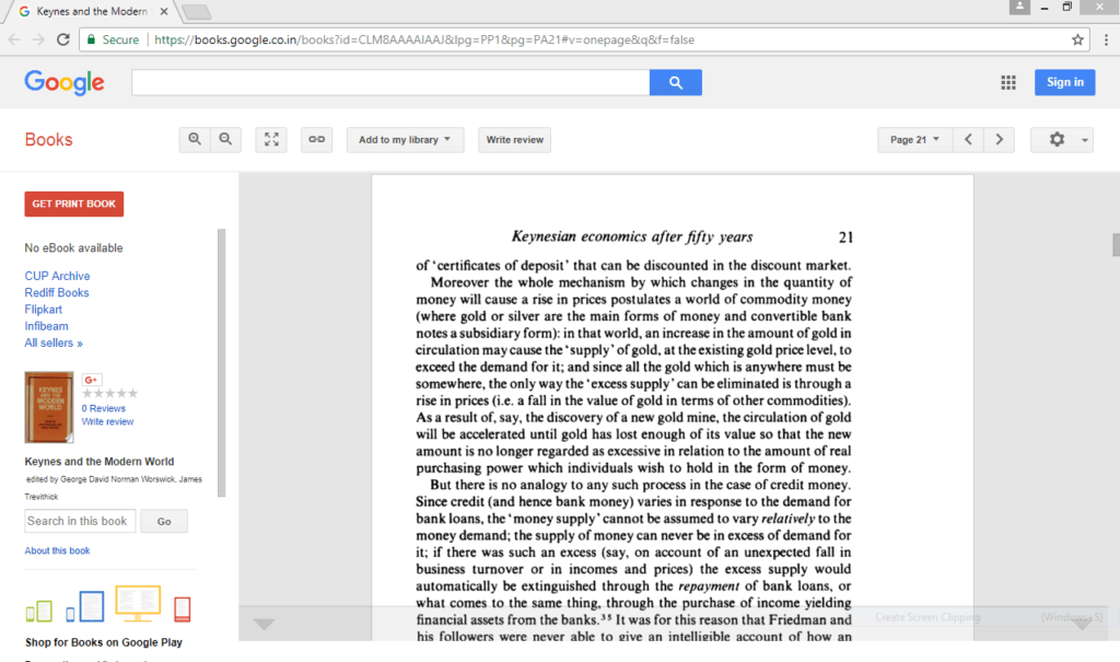
In his essay Keynesian Economics After Fifty Years, (in Keynes And The Modern World, ed. George David Norman Worswick and James Anthony Trevithick, Cambridge University Press, 1983), Kaldor wrote:

The excess supply would automatically be extinguished through the repayment of bank loans, or what comes to the same thing, through the purchase of income yielding financial assets from the banks.

Here’s the Google Books preview of the page:

click to view on Google Books

In his article, Circuit And Coherent Stock-Flow Accounting, (in Money, Credit, and the Role of the State: Essays in Honour of Augusto Graziani, 2004. Google Books link) Marc Lavoie showed how this precisely works using Godley’s transactions flow matrix. (Paper available at UMKC’s course site). See Section 9.3.1

The fact that the supply of credit and demand for money appeared to be independent

 … has led some authors to claim that there could be a discrepancy between the amount or loans supplied by banks to firms and the amount or bank deposits demanded by households. This view of the money creation process is however erroneous. It omits the fact that while the credit supply process and the money-holding process are apparently independent, they actually are not, due to the constraints or coherent macroeconomic accounting. In other words, the decision by households to hold on to more or less money balances has an equivalent compensatory impact on the loans that remain outstanding on the production side.

So if households wish to hold more deposits, firms will have to borrow more from banks. If households wish to hold less deposits, they will purchase more equities (in the model) and hence firms will borrow lesser from banks and/or retire their debt toward banks.

Other References

  1. Lavoie, M. 1999. The Credit-Led Supply Of Deposits And The Demand For Money – Kaldor’s Reflux Mechanism As Previously Endorsed By Joan Robinson, Cambridge Journal Of Economics. (journal link)
  2. Kaldor N. and Trevithick J. 1981. A Keynesian Perspective On Money, Lloyd’s Bank Review.

Open Mouth Operations

In the previous post Is Paul Krugman A Verticalist?, I discussed the confusions economists and market commentators have on open market operations. Even top economists such as Krugman suffer from confusions on central banking and monetary matters.

I also mentioned the work of Alfred Eichner on bringing out more clarity on the defensive nature of open market operations. Let’s look at these matters more closely.

Before this let’s look at what people in general think. Most people think of open market operations as some kind of extra activity on the part of the central bank in collaboration with the bureau of engraving and printing and think of it as operational implementation of Milton Friedman’s helicopter drops! So when a central bank such as the Federal Reserve changes its target on interest rates – such as lowering the “Fed Funds target rate”, people start commenting as if the Federal Reserve is undertaking a mystical operation.

This is Monetarist or Verticalist intuition. It is easy to show that open market operations have nothing to do with fiscal policy and as we saw in the previous blog – very little with monetary policy itself. The open market operation of the central bank is not an income/expenditure flow such as government expenditure flows or tax flows and the former does not affect the net worth of the change the net worth of either the domestic private or the foreign sector. Hence it is hardly fiscal. Yet commentators and economists keep arguing that the central bank is “injecting money” into the economy!

Even Paul Krugman erred on some of these matters and was shown how to do good economics by Scott Fullwiler in his post Krugman’s Flashing Neon Sign. Missing everything Fullwiler was saying, Krugman wrote another post A Teachable Money Moment which has the following diagram:
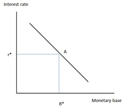
Below we will see how Krugman’s Neoclassical/New Keynesian (whichever) intuition is flawed.

Setting Interest Rates

These matters (the public understanding) have become worse ever since the Federal Reserve and other central banks around the world started purchasing government debt in the open markets on a large scale – in programs called Large Scale Asset Purchases (also called “QE”). In the following I will consider cases when there is no “asset purchase program” by the central bank and tackle this issue later in another post.

A simple case to highlight how a central bank defends an interest rate (as opposed to changing it) is considering the corridor system. There target for overnight rates is usually at the midpoint of this “corridor”. At the lower end of the corridor banks get paid interest on their settlement balances they keep at the central bank while at the upper end it is the rate at which the central bank lends.

Because banks settle among each other on the books of the central bank, this gives the latter to fix the short-term rates and indirectly influence long term rates.

Why do banks need to settle with each other?

One of the first economists to understand the endogenous nature of money was Sir Dennis Holme Roberston who used to work for the Bank of England. In 1922, he wrote a nice book simply titled Money.

 From page 52:

. . . If A who banks at bank X pays a cheque for £10 to B who banks at bank Y, then Bank Y, when it gets the cheque from B, will present it for payment to Bank X: and bank X will meet its obligation by drawing a cheque for £10 on its chequery at the Bank of England. As a matter of fact, the stream of transactions of this nature between big banks is so large and steady in all directions that the banks are enabled to cancel most of them out by an institution called the clearing-house:  but the existence of these chequeries at the Bank of England facilitates the payment of any balance which it may not be possible at the moment to deal with in this way …

Because banks finally settle at the central bank finally, central banks have learned since their creation that they can set interest rates. This is strongest at the short end of the “yield curve” but directly or indirectly central banks also influence long term rates.

At the end of each day, some banks will be left with excess of settlement balances (if they see more inflows than outflows) and some banks will face the opposite situation. Because they need to satisfy a reserve requirement at the central bank (which can be zero as well), some banks would need to borrow funds from others. Borrowing means paying back with interest and this is where the central bank’s ability to target rates comes enters the picture.

For suppose some bank X needs funds and other banks wish to lend bank X at a very high interest rate. In this scenario bank X can simply borrow from the central bank, while other banks who demanded higher interest will see themselves with excess settlement balances earning less than the target rate. So it would have been better for the latter to have lent than keep excess balances. (Of course the qualifier is that these things are valid under scenarios when there is less stress on the financial system). Also with the same logic, the rate at which banks lend each other will not fall below the corridor because it will be foolish of a bank to have lent settlement balances to another bank when it could have earned higher by just keeping excess settlement balances at the central bank.

Here is a diagram from the post Corridors And Floors In Monetary Policy from FRBNY’s blog which explains central bank’s operations:
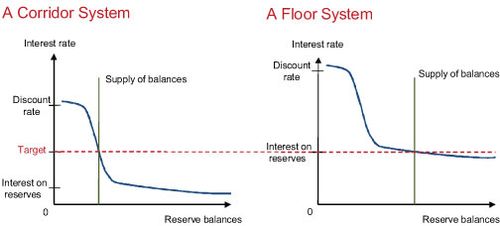
The other system as per this post is the floor system – in which the central bank’s target is the interest paid on settlement balances itself, rather than the midpoint of any corridor. This is what has been followed by the US Federal Reserve in recent times.

Back to the corridor system, an important question arises. Hopefully the reader is convinced that the overnight rate at which banks lend each other is between the corridor. However it is still unclear how and why the central bank can keep it at the midpoint.

If the central bank and the bankers understand the system well, it is possible for the central bank to be quite perfect in this. This happens for example in the case of Canada, where the bank is quite accurate in its objective.

The reason is that the central bank can easily add and subtract settlement balances by various means.

Take an example. Suppose the interest on reserves is 2.25%, the target is 3.00% and the discount rate – the rate at which the central bank lends overnight – 3.75%. If the central bank observes that banks are lending each other at 3.25% – slightly away from the target of 3.00%, it can simply create excess balances. Among the many ways, there are two –

  1. purchase/sale of government securities and/or repurchase/reverse repurchase agreements.
  2. shifts of government deposits from the central bank account into the Treasury’s account at banks or the opposite.

So the central bank knows how the curve in the figure above looks like and adds/subtracts settlement balances by the above methods (mainly). So banks are lending each other at 3.25%, the central bank will add settlement balances; if they are lending each other at 2.75% – the central bank will drain settlement balances.

More generally the “threat” by the central bank is reasonably sufficient to make banks lend at the target!

Open Mouth Operations

Let us suppose the central bank had been targeting 3.00% for three months now and decides to decrease rates.

What does it do?

Almost nothing!

The announcement itself will make banks gravitate toward the new target!

In his paper Monetary Base Endogeneity And The New Features Of The Asset-Based Canadian And American Monetary Systems, Marc Lavoie says:

When they [central banks] are not accommodating—that is, when they are pursuing “dynamic” operations as Victoria Chick (1977, p. 89) calls them—central banks will increase (or decrease) interest rates. As shown above, to do so, they now need to simply announce a new higher target overnight rate. The actual overnight rate will gravitate toward this new anchor within the day of the announcement. No open-market operation and no change whatsoever in the supply of high-powered money are required.

Hence the term “open mouth operations” which was coined by Julian Wright and Greame Guthrie in their paper Market-Implemented Monetary Policy with Open Mouth Operations.

Open Market Operations

The above paper by Marc Lavoie is an excellent source for open market operations and looking at central banking from an endogenous money viewpoint.

I mentioned in the previous post that the open market operations are defensive. In my analysis in this post till now, I ignored the factors which cause settlement balances of the banking sector as a whole to change. Let us bring in this complication.

Apart from banks, the Treasury – the domestic government’s fiscal arm – and other institutions such as foreign central banks, governments and international official institutions (such as the IMF) also keep an account at the (domestic) central bank. When these institutions transact, there is an addition/subtraction of banks’ settlement balances at the central banks.

Here’s one example. Suppose the Treasury transfers funds of $1m to a contractor for settlement of a project done by the latter. When the funds are transferred, the contractor’s bank account increases by $1m and the bank in which he banks sees its deposits and settlement balances rise by $1m while the central bank will reduce the Treasury’s deposits by $1m.

This may lead to a deviation of banks’ lending rate to each other and the central bank needs to drain reserves. The central bank can achieve this by shifting government funds at a bank into the central bank account. If the central bank transfers $1m of funds, banks’ deposits and settlement balances reduce by $1m and the Treasury’s account at the central bank will increase by $1m.

This is not an “open market operation” but another way of adding/draining reserves. In general, depending on institutional setups, the central bank may also do purchase/sale of government securities and/or repurchase agreements.

But this has nothing to do with policy itself – rather it is to maintain status quo. (Of course “large scale asset purchases” is a slightly different matter – first one needs to understand the corridor system).

In other words, this is a defensive behaviour on part of the central bank.

Alfred Eichner

In the previous post and in Alfred Eichner And Federal Reserve Operating Procedures, I mentioned about the contribution of Eichner. In an essay in honour, Alfred Eichner, Post Keynesians, And Money’s Endogeneity – Filling In The Horizontalist Black Box, (from the book Money And Macrodynamics – Alfred Eichner And Post-Keynesian Economics) Louis-Philippe Rochon says:

For Eichner, the overall or “primary objective [of the central bank], in conducting its open market operations, is to ensure the liquidity of the banking system,” which applies to either the accommodating or defensive roles. In either case, Eichner argues that “the Fed’s open market operations are largely an endogenous response to . . . the need both to offset the flows into and out of the domestic monetary-financial system and to provide banks with the reserves they require”; that is, resulting from the demand for money and the demand for credit respectively (1987, 847, 851).

And while the accommodating argument has been debated at length by post-Keynesians, the defensive role has been virtually ignored and only recently rediscovered (see Rochon 1999). Yet it is certainly Eichner’s greatest contribution to the post-Keynesian theory of endogenous money. . .

. . . The “defensive” behavior is defined by Eichner as the “component of the Fed’s open market operations [consisting] of buying or selling government securities so that, on net balance, it offsets these flows into or out of the monetary-financial system,” leaving the overall amount of reserves unchanged. This is the result of changes in portfolio decisions and increases or decreases in bank (demand) deposits. As a result of an increase in the nonbank’s desire to hold currency, for instance, “in order to maintain bank reserves at the same level, the Fed will need to purchase in the open market government securities equal in value to whatever additional currency the nonbank public has decided to hold” (Eichner 1987, 847).

In making the distinction between temporary and permanent open market operations, Rochon also quotes Scott Fullwiler:

Outright or permanent open market operations are primarily undertaken to offset the drain to Fed balances due to currency withdrawals by bank depositors. . . . Temporary open market operations are aimed at keeping the federal funds rate at its target on average through temporary additions to or subtractions from the quantity of Fed balances. Temporary operations attempt to offset changes in Fed balances due to daily or otherwise temporary fluctuations in the Treasury’s account, float, currency, and other parts of the Fed’s balance sheet, in as much as is necessary to meet bank’s demand for Fed balances. (2003, 857)

Paul Krugman

All this is completely opposite of Paul Krugman’s position that

. . . And currency is in limited supply — with the limit set by Fed decisions.

And Krugman’s mistake is not minor – it seems he is completely unaware of the huge difference money endogeneity makes.

So what is the difference between Krugman’s diagram and the one from FRBNY blog – even though they look similar? The difference is that the latter is descriptive of behaviour when policy is unchanged and is useful for describing open market operations etc while Krugman uses the same to describe policy changes – which in reality happen via open mouth operations. Paul Krugman confuses open market operations and open mouth operations. So much for a “teachable money moment”.

Krugman also shows his Monetarist intuition by claiming:

And which point on that curve it chooses has large implications for the economy as a whole. In particular, the Fed can always choke off a private-sector credit boom by moving up and to the left.

implying that the central bank in reality controls the monetary base and thence the money stock.

Some Post Keynesians argued since long ago that the central bank cannot control the money stock:

Here’s on Wynne Godley from from The Times, 16 June 1978:
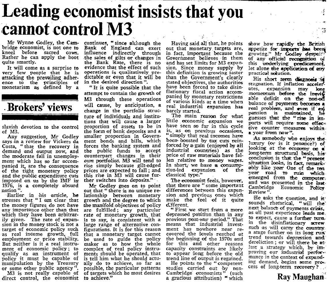
(click to enlarge)
Is Paul Krugman A Verticalist?

24 years back, Basil Moore wrote a book Horizontalists And Verticalists: The Macroeconomics Of Credit Money (Cambridge University Press, 1988) which begins like this:

The central message of this book is that members of the economics profession, all the way from professors to students, are currently operating with a basically incorrect paradigm of the way modern banking systems operate and of the causal connection between wages, prices, on the one hand, and monetary developments, on the other. Currently, the standard paradigm, especially among economists in the United States, treats the central bank as determining the money base and thence the money stock. The growth of the money supply is held to be the main force determining the rate of growth of money income, wages, and prices.

… This book argues that the above order of causation should be reversed. Changes in wages and employment largely determine the demand for bank loans, which in turn determine the rate of growth of the money stock. Central banks have no alternative but to accept this course of events, their only option being to vary the short-term rate of interest at which they supply liquidity to the banking system on demand. Commercial banks are now in a position to supply whatever volume of credit to the economy their borrowers demand.

The book built on his own work and that of Nicholas Kaldor and Marc Lavoie among others goes on to describe the banking system, horizontalism and endogenous money. Money is credit-led and demand-determined was his message. Economists believing in the “incorrect paradigm” are Verticalists in Moore’s terminology.

Paul Krugman whom Post Keynesian have more respect than other mainstream economists probably disappointed them when he was arguing with Steve Keen in a 3-post blog series. Arguing like a Verticalist, Krugman claims (among other Verticalist claims) in his post Banking Mysticism, Continued:

… And currency is in limited supply — with the limit set by Fed decisions. So there is in fact no automatic process by which an increase in bank loans produces a sufficient rise in deposits to back those loans, and a key limiting factor in the size of bank balance sheets is the amount of monetary base the Fed creates — even if banks hold no reserves.

The Defensive Nature Of Open Market Operations

The reason there is widespread misunderstanding of what the central bank does is because it carries out open market operations where it buys or sells government securities or does repurchase agreements. The orthodox view is that the central bank is acting the way it is to increase or decrease the amount of banks’ settlement balances and this affects the money supply – allowing banks to expand lending or leading them to contract – and thence the whole economy. The view is that the central bank has a direct control these operations and are purely volitional.

This is an incorrect view because no central bank claims to be “controlling” the money stock.

If money is truly endogenous, the question is why the central bank does these operations often. The reason is that operations of the central bank are defensive. 

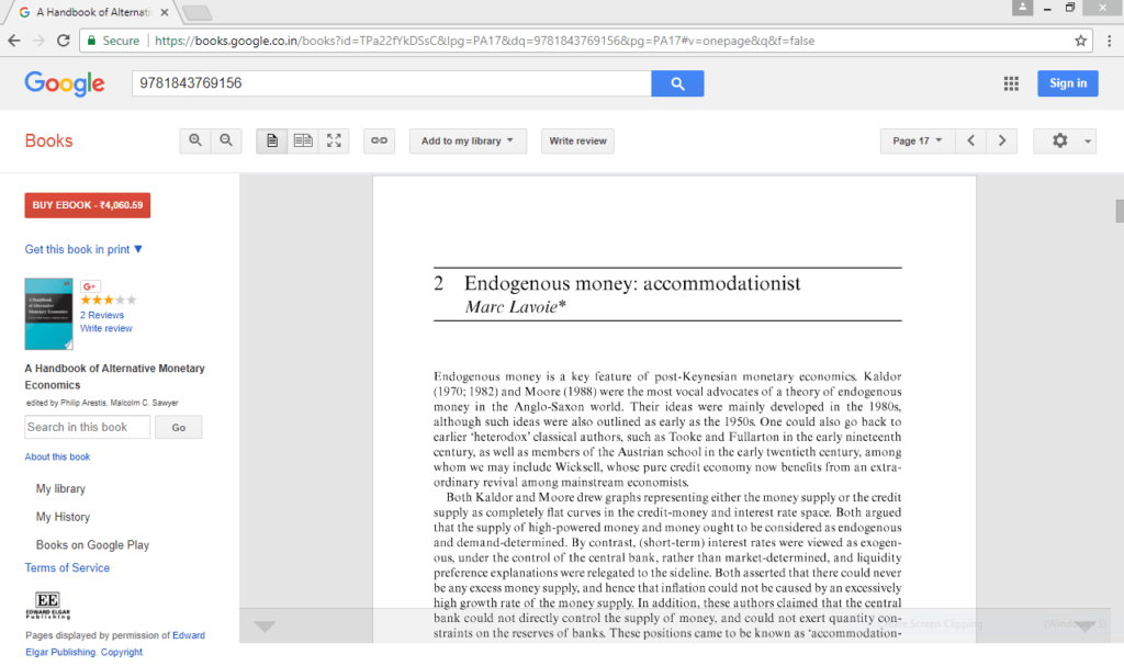
In his article Endogenous Money: Accomodationist, Marc Lavoie argues:

Some post-Keynesians have pointed out long ago that open market operations had little or nothing to do with monetary policy.

For instance, It is usually assumed that a change in the Fed’s holdings of government securities will lead to a change, with the same sign attached, in the reserves of the commercial banking system. It was the failure to observe this relationship empirically which led us, in constructing the monetary financial block of our model, to try to find some other way of representing the effect of the Fed’s open market operations on the banking system. (Eichner, 1986, p. 100)

That other way is that ‘the Fed’s purchases or sales of government securities are intended primarily to offset the flows into or out of the domestic monetary-financial system’ (Eichner, 1987, p. 849).

So the central bank purchases government bonds and/or does repos to neutralize the effects of transactions which change the settlement balances. One example is the flow of funds into and out of the government’s account at the central bank. Another is the demand for currency notes by banks to satisfy their customers’ needs. The central bank has no choice but to provide these notes.

Here’s a preview via Google Books:

click to view on Google Books

Also see this post Alfred Eichner And The Federal Reserve Operating Procedures.

Krugman is partly right when he says, “Banks are important, but they don’t take us into an alternative economic universe.” However he fails to see that money is endogenous and the way the banking system works show this endogeneity.

Of course, Steve Keen has issues with his models and accounting with which Krugman has troubles. Keen defines aggregate demand to be gdp plus “change in debt”. As much weird this definition is, it is double counting when investment expenditure is financed by borrowing rather than internal sources of funds. Also, if a person sells a home to another person who has financed this purchase by borrowing and the former does not make expenditure from this income, this does not increase aggregate demand – a point raised by Marc Lavoie here (h/t “Circuit” from Fictional Reserve Barking). But as per Keen’s definition it does. In his first post, Krugman seems to say the same thing as Lavoie – but in a roundabout way.

The resulting debate has however highlighted the Verticalist intuition of Krugman!

More National Accounts: Consumption Of Fixed Capital

In one of my recent posts, Saving Net Of Investment, I went into gross saving versus saving net of consumption of fixed capital. I showed how depreciation – or more appropriately, consumption of fixed capital – is treated in the flow of funds accounts.

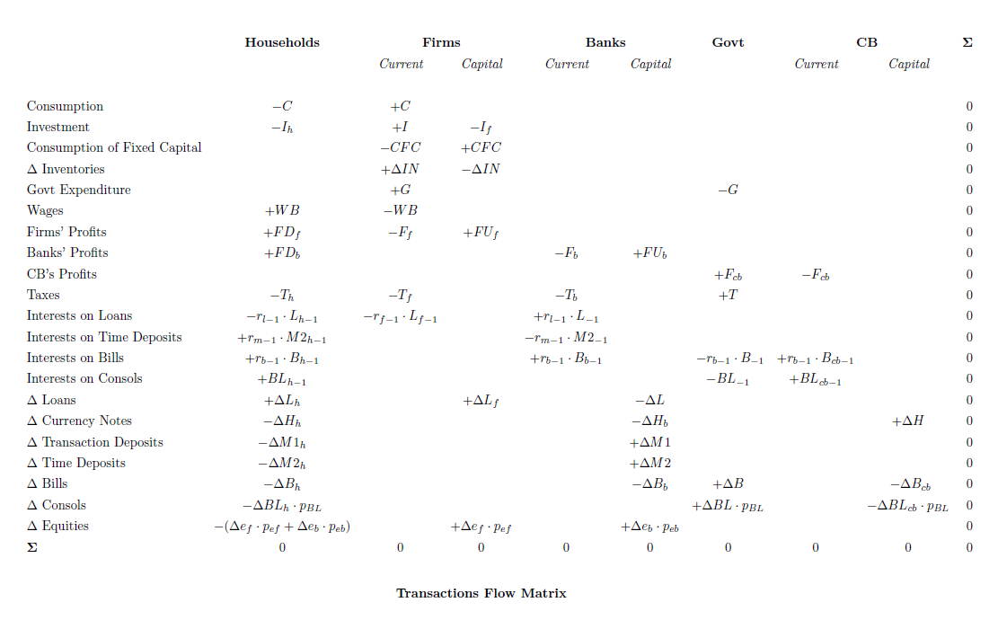
Since the transactions flow matrix is a powerful tool for visualizing flow of funds, the question is where depreciation makes an appearance. The following table created by me using shows how for a simple economy.

FIGURE 1. Transactions Flow Matrix (click to enlarge)

Here “Firms” is a shorthand for all production firms as a sector and I took the consumption of fixed capital of firms only for illustration purposes. (Else I would have needed to break the households’ accounts into current and capital accounts – eating up space).

Investment here is gross investment and consumption of fixed capital makes its appearance in the line 3. It is a negative item in the current account and a positive item in the capital account. So it more of a book-keeping device but an important one because depreciation is not unimportant. The definition of profits is that of Wynne Godley and is slightly different from National Accounts. Also, while undistributed profits is a source of funds, CFC is also!

In my posts Net Worth and Net Worth: Part 2, I went into how net worth is defined. Also for a background on sources and uses of funds, see this post Sources And Uses Of Funds.

So undistributed profits (FU) and consumption of fixed capital (CFC) are both sources of funds. (Positive signs denote sources of funds and negative – uses of funds). This can be confusing because depreciation is a negative for net worth. The reason is that, as I have mentioned before, revaluations need to be done before end of period stocks are calculated. And it is where consumption of fixed capital will make a reappearance – subtracting from net worth due to a reduction in the value of nonfinancial assets.

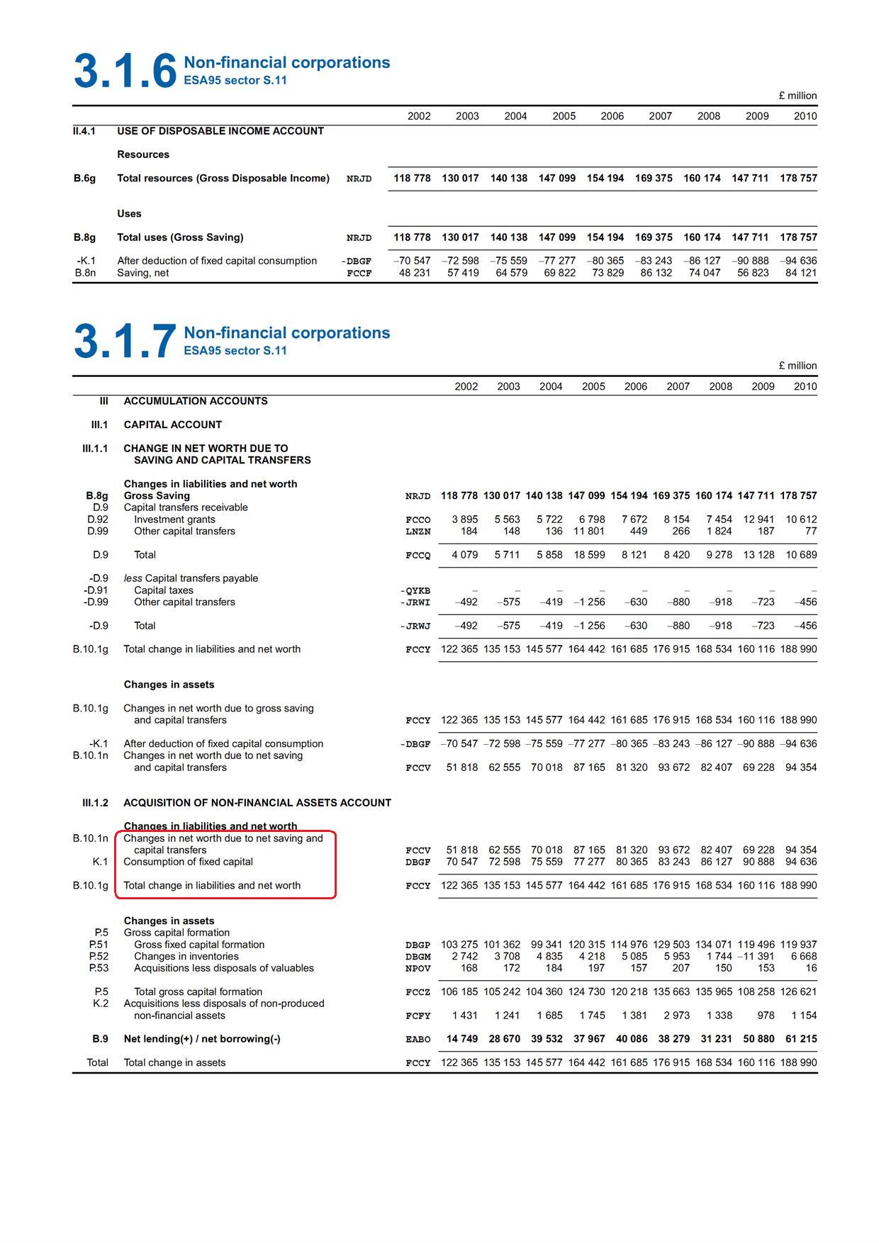
It is important to keep in mind that equities are also sources of funds as the last line (above Σ) shows. So net saving (undistributed profits for firms) and consumption of fixed capital add to changes in net worth. (Note: Net is net of consumption of fixed capital here and not net of investment!).

This can be seen from the UK Blue Book 2011.

FIGURE 2.  UK Blue Book 2011 Accumulation Accounts (click to enlarge)

A Digression

What is the origin of the confusing phrase “net saving” – saving net of investment? I believe it came from Nicholas Kaldor himself who originated the sectoral balances approach. Here’s from The Scourge Of Monetarism, 1982, pp 48-50:

The PSBR in any year can be defined as the public sector’s net de-cumulation of financial assets (net dissaving) which by accounting identity must be equal to the net acquisition of financial assets (net saving) of the private sector, home and overseas; which in turn can be broken down to the net acquisition of financial assets of the personal sector, of the company sector, and the overseas sector (the latter is the negative of the balance of payments on current account).

Debt Sustainability

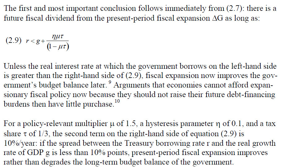
In a recent paper, Bradford DeLong and Lawrence Summers suggest that a fiscal expansion can be useful to bring an economy from a depressed state (!). The rough idea being that a relaxation of fiscal policy leads to a higher output and the increase in economic activity leads to a stabilization of public debt/gdp ratio.

This condition is valid as long as (in the authors’ terminology):

(click to enlarge)
The interesting thing about this is that the authors suggest that even if r > g, it is possible for the public debt/gdp to remain sustainable under certain conditions.

I won’t have more to say on this because it uses a standard one-period analysis but the fact that some mainstream authors seem to understand the fiscal policy dynamics better is encouraging.

Of course, this result was known to Post Keynesians – Wynne Godley and Marc Lavoie showed this in this paper Fiscal Policy In A Stock-Flow Consistent (SFC) Model (pay-walled, for the working paper click here).

Arguing that their “… conclusions conflict with those of the “new consensus,” which holds that a correct setting of interest rates is the necessary and sufficient condition for achieving noninflationary growth at full employment, leaving fiscal policy rather in the air.”, they also derive a result for a closed economy:

It is usually asserted that, for the debt dynamics to remain sustainable, the real rate of interest must be lower than the real rate of growth of the economy for a given ratio of primary budget surplus to gdp. If this condition is not fulfilled, the government needs to pursue a discretionary policy that aims to achieve a sufficiently large primary surplus. We can easily demonstrate that there are no such requirements in a fully consistent stock-flow model such as ours.

The G&L style of modeling is extremely useful because it gives great attention to stocks and flows so that no errors creep in. The result is surprising the first time one hears this because it goes against intuition. This can be seen by thinking of the interest payments of the government as income for the domestic private sector!

So no conditions such as r < g!

Open Economy Debt Dynamics

For open economies, G&L are also able to construct select scenarios where a debtor nation can be indebted to the rest of the world without the nation’s debt (which is different from public debt) increasing relative to gdp forever. (Of course by no means proving/implying it for all possible scenarios).

So let us consider the debt dynamics equation (see A Practical Guide To Public Debt Dynamics, Fiscal Sustainability And Cylical Adjustment of Budgetary Aggregates from the IMF, which can be equally applied to the open economy case)

where d is “external debt” and pb is the primary balance of the current account balance. (The expressions are relative to gdp)


Suppose the government and the central bank want to restrict external debt to 50% of gdp – with the view that foreigners may consider moving above it as unsustainable. Assume growth is 3.5% and effective interest rate paid on liabilities to foreigners is 1%. Then the tolerable primary deficit of current account balance is 1.25%. This is calculated by setting the left hand side to zero and just plugging the formulas. (See below)

Please note, a higher growth will worsen the external balance so it is not a good argument that growth can lead to a lower debt/gdp ratio.

To summarize, intuitions for a closed economy and the open economy can appear contradictory.

Standard Analysis

I have seen many economists including Post Keynesians (not G&L) take the above equation and interpret it rather differently. So assuming sustainability, a constant primary balance pb implies the debt sustains at

or simply,

A continuous time formulation leads to an equality sign. The above is derived by assuming the debt sustains at d and shuffling the terms in the first equation.

Note: the above is valid only if there a stabilization. Else, in the case where g < r, the above expression gives a negative answer for a negative primary balance – but that is because the derivation assumed sustainability and cannot be used when debt/gdp keeps rising.

This is also written sometimes as

by expanding the denominator of the previous expression using the Taylor Theorem from Mathematics.

This raises a curiosity – how come in the G&L case for the closed economy did the debt sustain even when g > r? That’s because it was a dynamic stock-flow consistent model as opposed to the artificial assumption of a constant deficit used in standard analysis such as the third equation above.

Nonetheless the above analysis shows that for a constant deficit (though artificial), debt sustains as per the equation (assuming growth and the rate of interest paid are constant as well!)

Back to Open Economies

Moving to the open economy case, where debt and deficit denote the external debt and the current account deficit, the above shows that if the primary deficit is restricted somehow to say 5% of gdp and the differential between growth and interest rate is 2%, the external debt sustains at 250% of gdp.

This should be seen as a restriction. Instead some/many Post Keynesians just state it is sustainable. A higher growth rate will increase the deficit (current account) and the debt-dynamics can make the whole process unsustainable. So one needs to model how fiscal policy itself affects the current account deficit rather than keeping it a constant relative to gdp.

This is the reason many nations find themselves troubled by the external sector.

This can be seen for the case of the United States. A huge relaxation of fiscal policy will bring back the current account deficit to 6% of gdp (and rising) and put the world on an unsustainable path. What the United States needs to do is ask its trading partners to expand domestic demand by fiscal expansion and achieve higher growth so that it itself can achieve a higher growth rate due to the extra space created for fiscal policy.

More generally, we need a concerted action!

For a related analysis see Dean Baker’s recent analysis on the trade deficit being America’s fundamental imbalance: The Iron Grip of Accounting Identities

Summary

There is no condition such as if r <g, debt is sustainable. Debt can keep rising relative to gdp simply because deficit keeps rising.

The condition r > g can be useful in studying certain circumstances for analysis.

Some Monetary Facts

Money is endogenous and is created as a byproduct of the production process. I came across this reference which supposedly shows that there is supposedly a one-to-one relationship between money and inflation and hence as a consequence – if we were to believe this – if the Bureau of Engraving and Printing were to work extra-time, this would lead to high inflation!

This is a highly misleading. Borrowing to produce something leads to an increase in demand and wealth and the private sector allocates its financial wealth into deposits and various securities. So money is a residual. Some of the increase in demand spills over to price rise and in exceptional cases can run out of control because of other reasons as well, leading to more borrowing and hence a growth in the money stock and higher inflation. But it is misleading to say that the growth of the money stock caused the inflation.

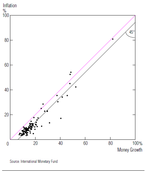
The reference is Some Monetary Facts from the Summer 1995 Quarterly review of the Federal Reserve Bank of Minneapolis which makes confusing statements about what the central bank does or should do. Here’s a graph from the paper supposedly establishing a connection between growth in the money stock and inflation. I added the pink line to make it look less scary 🙂


The points in the graph are average growth rates of the money stock and price rises for 110 countries.

According to the authors, the correlation is around 0.95 and the 45° line supposedly shows the tight link between money and inflation.

God we are in for a very high inflation soon!

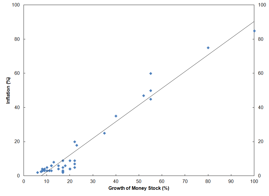
This correlation analysis can easily be produced by creating a data set with the same properties (high correlation, 45 degree line etc) and I was able to do so below:

 The slope is nearly 1 (0.97) and a correlation of 0.97 (even better!).

When you look at the individual data, you will see that except countries with very high inflation, there is hardly any issue.

Here’s the excel sheet Money And Inflation.

If you were to remove the points with high inflation, the “monetary facts” as per the authors go away.

Of course, did money (or central bank open market operations) cause inflation in those countries – of course not. Money is a residual.

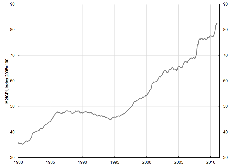
How does the M2/CPI look for the United States? Here’s the monthly graph of the ratio, with M2 in billions of dollars and CPI defined so that is equal to 100 in 2005. This following shows how wrong the “Monetarist intuition” is. Money didn’t increase one-to-one with prices and the ratio has grown from 35.8 to 82.7.

(Data Source: Federal Reserve Bank of St. Louis)

Note: The data in the excel sheet was created using random data and some amount of tweaks by me to reach the graph similar to the original Minneapolis Fed paper. So it is an imaginary data set created to have similar properties.

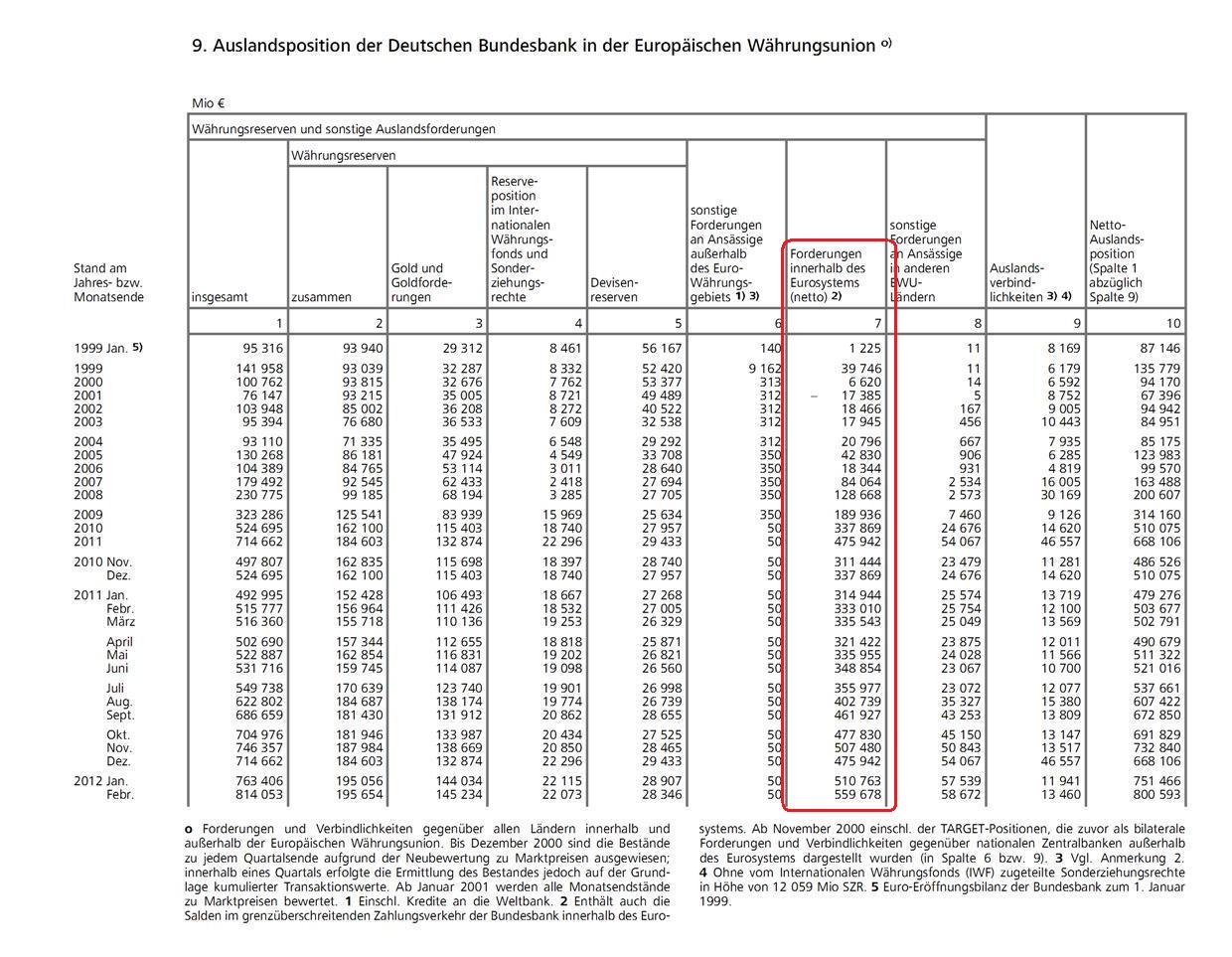
Deutsche Bundesbank’s TARGET2 Claims: Again!

At the risk of boring readers, here’s Bundesbank’s TARGET2 claims again from its March 2012 Monthly Report. Cannot find the English version but the translation is below the first figure (with old data). This increased to almost €560bn at the end of February despite ease in financial market conditions in the Euro Area!

(click to enlarge)
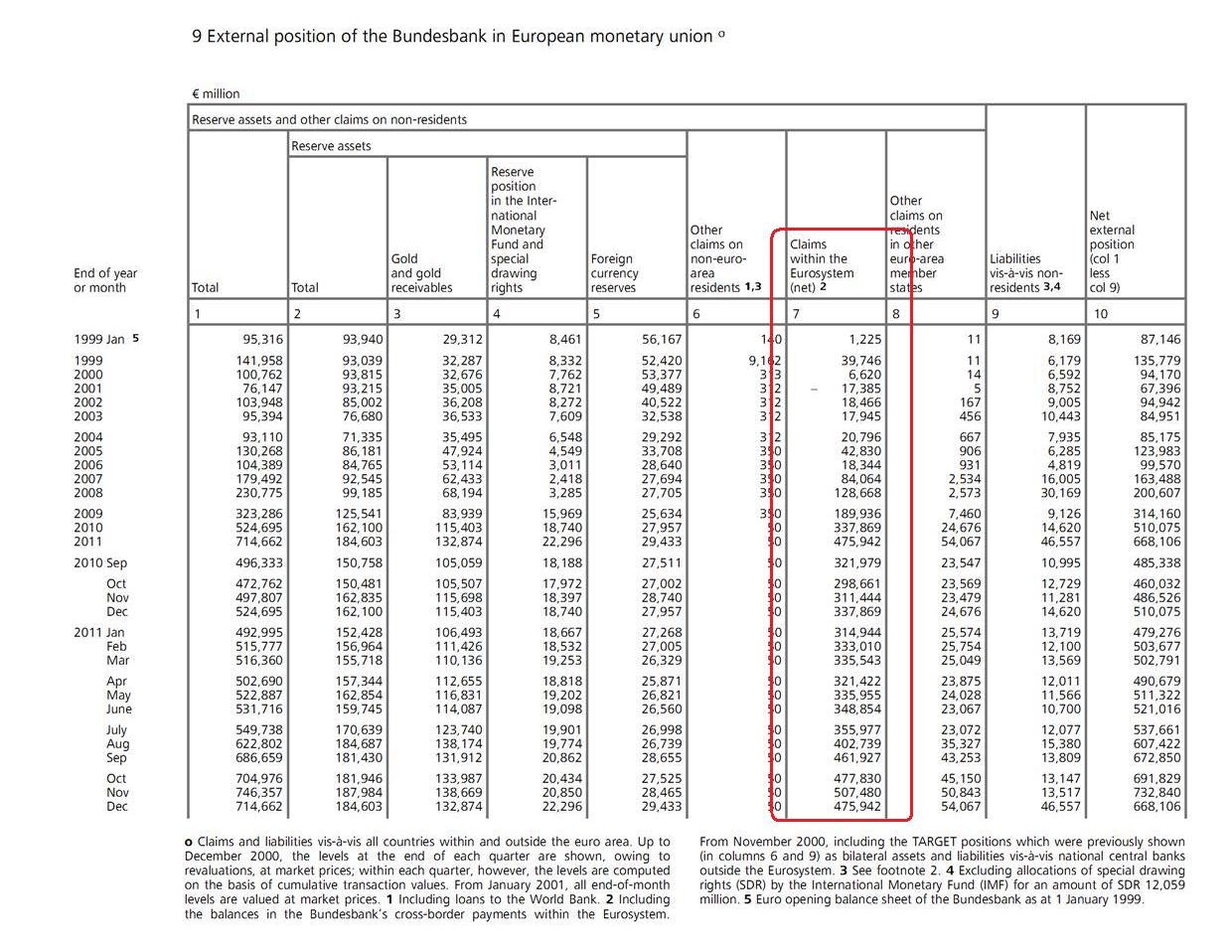
English translation from an older report:

(click to enlarge)

As mentioned earlier these arise due to capital flight into Germany from the “periphery” countries.

Some economists and financial analysts try to downplay this by saying that in reality the actual loss (in case of a breakup of the Euro Area and subsequent default by the periphery) to Bundesbank and hence Germany is lesser and this number should be multiplied by the capital key. For Bundesbank this is 18.9373% and using the February number this amounts to a maximum loss of €106bn as per this calculation.

This is misleading to the core. Firstly if the debtor nations default the creditor nations suffer in full. So if Bundesbank’s losses are low, other creditor nations’ losses will be high. Also, Bundesbank suffers due to losses incurred by other NCBs of creditor nations such as Belgium since these losses are shared. Secondly, the capital key would be some sort of weighted key among the creditor nations’ central banks and will be higher.

At any rate, the creditor nation lose the full amount of the claim of the ECB on the periphery nations in the case of a breakup. This number can vastly increase if there is a panic and further capital flight into the “core”. Of course, there will be other losses and costs of a breakup but IMO – nonetheless this is not unimportant.

Having said this, these things are very unpredictable – it is perfectly possible that a boom in financial markets for whatever reasons reverses the flight making the unsustainable process run longer than one may think. It is also possible – as Euro Area leaders have been planning wittingly or unwittingly – that trade is balanced internally by deflating demand in debtor nations and but this will come with a lower output and higher unemployment in general and injures all alike.

The above increase could also have been because banks in nations such as Spain may have redeemed some of their liabilities to banks in Germany and refinanced themselves via the three-year LTRO in February.

Saving Versus Saving Net Of Investment

The commenter JKH has an outstanding post here at Cullen Roche’s blog criticizing the Neochartalists’ mixing up of saving and saving net of investment.

JKH quoting Randy Wray:

Then, this is telling:

“To briefly summarize, at NEP we prefer to use the Godley sectoral balance approach, where he defined private sector saving as “net accumulation of financial assets” (NAFA), using the flow of funds data. Typically economists use the GDP equals national income equation where saving is defined as a residual: the net income received but not consumed (I’ll use it below in discussing the MMR approach). In theory these would lead to approximately the same result; in practice they do not because the NIPA accounts include imputed values. Godley preferred the flow of funds data but even they had to be carefully adjusted to ensure that every spending flow is actually financed and actually “goes somewhere” (ensuring “stock-flow consistency”). That is all quite wonky. My bigger point is that we can come up with alternative definitions of saving that would include unrealized capital gains as real and financial assets appreciate in value.”

This seals the case regarding MMT’s confused interpretation of the term “saving”. I don’t know if that correctly reflects what Godley does or not, but if private sector saving is defined that way it has nothing to do with the private sector saving S that’s cast in MMT’s own 3 sector financial balances model. S cannot identically equal (S – I) unless I is identically zero, which is ridiculous.

For example, in a closed economy with a balanced budget, if the (alleged) Godley definition of private sector saving is combined with the explicit definition of private sector saving S in the 3 sector SFB equation, then saving must be identically zero, whatever the level of investment. In cannot be otherwise for the Godley and MMT SFB specifications of S to be consistent. And in the real world economy, any such consistency would force global S = 0. And this is the point of it all – such inconsistency in the use of the term “saving” is fundamentally misleading.

Remarkably, Wray just demonstrated the same conflation of saving and net saving in MMT language and logic that is at the heart of the issue in question, which I find flabbergasting in the circumstances. Furthermore, he suggests this is consistent with the NIPA definition of saving. The definition of saving (allegedly) attributed to Godley above is not the same as NIPA defined saving at all. And the issue of imputed values or capital gains has nothing to do with the primary question. That is a secondary consideration having to do with the reconciliation of stocks and flows, not the outright confusion of flow definitions. It is a trees rather than a forest issue.

Of course this is an erroneous application of Godley’s sectoral financial balances approach as JKH himself suspects.

Wynne Godley never

… defined private sector saving as “net accumulation of financial assets” (NAFA), using the flow of funds data

and always specified that it is Net Saving which is NAFA and always specified Net Saving is Saving Net of Investment.

Excellent post by JKH exactly pinpointing to mixing terminologies and taking great pains to explain saving as an income residual.

JKH on me

Special mention also goes to Ramanan, who is a persistent seeker of accuracy when it comes to the subject more generally.

Thank you 🙂