Tag Archives: flow of funds

Link

New UK Flow Of Funds

The UK Office Of National Statistics (ONS) is planning to publish new flow of funds statistics in the future. Till now, the ONS had just the SNA tables. Although the SNA has lots of details on stocks and flows, flow of funds gives more details.

ONS summary:

See our first combined set of experimental flow of funds statistics using new data sources providing improved breakdowns of how money moves around the UK economy

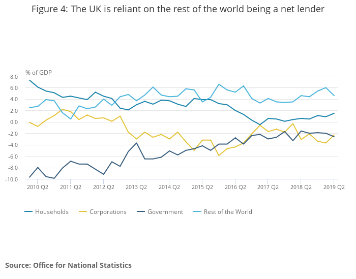
The article also has a discussion on sectoral balances which has the chart on top of this post.

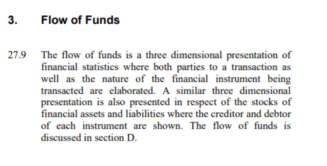
The 2008 SNA explains this:

A New Way To Learn Economics?

John Cassidy has a nice article titled A New Way To Learn Economics for The New Yorker on a new online introductory economics curriculum. produced by a lot of collaborators.

I went to the website which has the full book. Although there seems to be some progress, I have a strong reservation against it.

The chapter titled “Banks, money and the credit market” has a much better description on it than textbooks widely used, such as the ones by Paul Samuelson, Gregory Mankiw or Paul Krugman. On a cursory look, I didn’t find anything about the “money multiplier” model. Instead, the book says that central banks set short term interest rates and this has an effect on aggregate demand. If I missed something and if you find something orthodox, please let me know.

The chapter on fiscal policy looks like being written by fiscal hawks. There is a description of the government expenditure multiplier, which is not much different from other textbooks. There’s no mention of the more complicated nature of this process because of interactions between stocks and flows. For example, in stock-flow coherent (SFC) models, this one-step multiplier has a limited role.

Now, fiscal policy has strong effects and the book hardly does justice to any of this. It reads more like a defense of the establishment wisdom.

But it is in the area of international trade and globalization under the current rules of the game that the book is the most disappointing. The authors do tell students that it can produce “losers” but the problem of such an approach is that it doesn’t appreciate the fact that it leads to polarisation and divergences in fortunes of nations, instead of individuals. The assumption and conclusion (the same thing in most of economics!) is that if losers are compensated, fortunes of nations can converge.

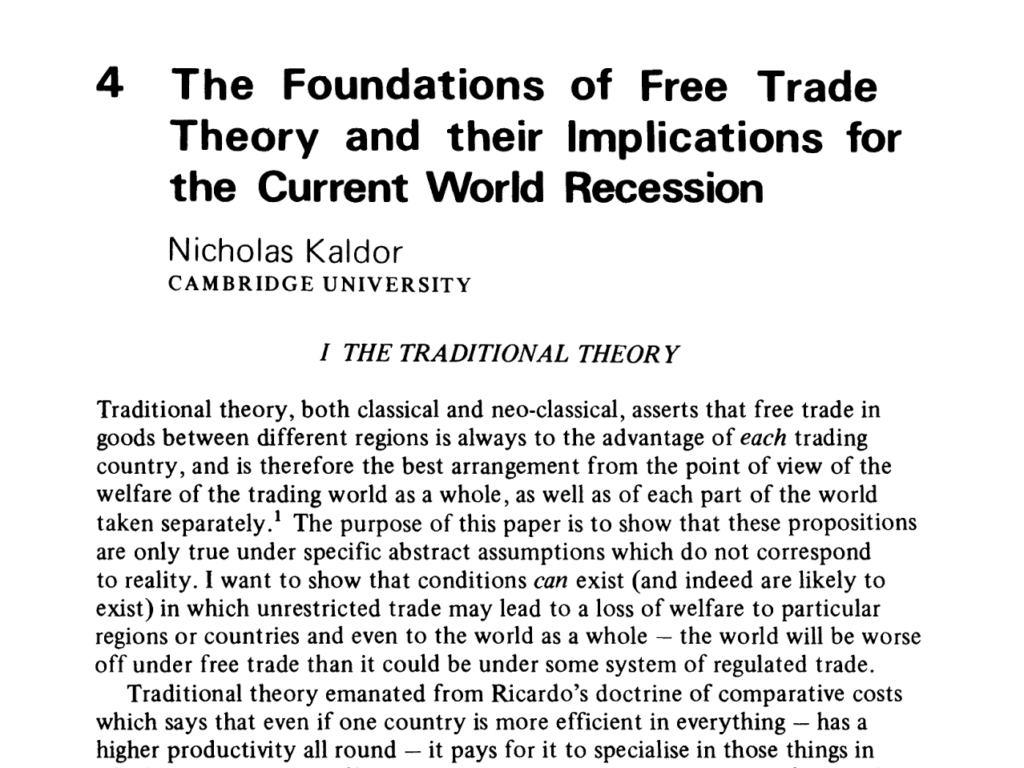
This by Nicholas Kaldor, written in 1980, is change.

Not the new book, The Economy. 

As Morris Copeland emphasised, the root problem of economics is the total confusion of anyone and everyone on what money is. And his approach shows us that it’s not complicated. One just needs to study flow-of-funds or social accounting. There is hardly any emphasis of this in the book. Till then, students will remain confused and ignorant about the way the world works.

Morris Copeland’s Monetary Economics

Morris Copeland was the discoverer (or inventor?) of the flow of funds approach. The U.S. Federal Reserve publishes the statistics every quarter but is largely ignored. Copeland was of the view that it is essential to get rid of myths in economics. He said:

The subject of money, credit and moneyflows is a highly technical one, but it is also one that has a wide popular appeal. For centuries it has attracted quacks as well as serious students, and there has too often been difficulty in distinguishing a widely held popular belief from a completely formulated and tested scientific hypothesis.  I have said that the subject of money and moneyflows lends itself to a social accounting approach. Let me go one step farther. I am convinced that only with such an approach will economists be able to rid this subject of the quackery and misconceptions that have hitherto been prevalent in it.

– in Social Accounting For Moneyflows, in Flow-of-Funds Analysis: A Handbook for Practitioners (1996) [article originally published in 1949]

In an article titled, Some Illustrative Analytical Uses Of Flow-of-Funds Data, in the book, The Flow-of Funds Approach To Social Accounting, published in 1962, he has several interesting things to say about the myths prevalent even among most economists.

Page 196:

The FOF accounts help to dispel various misconceptions in regard to the role of money and of other forms of credit in the income and money circuit. Among these misconceptions are such ideas as that: (1) it is safe to assume that private nonbank cash balances are mostly consumer cash balances; (2) the banking sector is more than a mere financial intermediary, that by itself it can “create” a substantial amount of “money” that can be used to finance a substantial increase in aggregate demand; (3) a government deficit in a particular year or other period can be considered inflationary without stopping to consider whether it represents a fiscal change from the preceding period that tends to increase aggregate demand or whether it occurs at a time when the economy is operating at or near or far below full capacity; and (4) when the government seeks to raise a large amount of money through financial channels to finance a war, one can ignore the fact that an excess of nonfinancial uses over nonfinancial sources of funds for the government means an equal excess of nonfinancial sources over nonfinancial uses of funds for the rest of the economy and a consequent equal amount of money that the rest of the economy will necessarily advance to the government through financial channels.

Note: in (2) above, Copeland is talking of finance of government deficit via sale to banks as compared to sale to the general public and these two have different effects on the money stock. Same below.

Page 197:

It is not easy for us today to imagine what it must have been like to try to understand the workings of our economy in the absence of social accounting information. The workings of those aspects that involve financial transactions seem to have been particularly difficult to understand. Indeed, I think we can say that in the absence of financial transaction social accounting information various misunderstandings were permitted to develop. Let me mention three:

  1. One of these relates to the role of trade credit in the business cycle. This is a subject that probably received somewhat less attention than it deserved fifty-odd years ago, but it seems to have greatly intrigued H. J. Davenport, and he came up with this curious conclusion about the contraction of credit during a commercial crisis— “Side by side with the diminution of bank credit there is taking place an enforced and inevitable expansion of credit relations between producers and consumers, producers and middle-men, and between middle-men and consumers.”
  2. During World War I Secretary of the Treasury W. G. McAdoo, among others, was greatly concerned about the possibility that the huge wartime increase in the demand for funds would drive interest rates sharply up. As a matter of fact, interest rates did rise but by no means as sharply as McAdoo had anticipated. Railroad bond yields rose from 4.12 per cent in April 1917 to 4.42 per cent in November 1918. During World War II the yields on long-term United States bonds actually declined.
  3. There is a view still entertained by quite a number of economists that an increment in the currency and deposit liabilities of the banking and monetary system creates a net addition to the total sources of funds available to finance purchases of GNP and so, a net addition to aggregate demand.

Page 207:

There is still another type of misconception that I hesitated to mention in my opening remarks because it is of a rather subtle nature. I would like to comment on it briefly at this point. Let me indicate its nature by quoting from George Leland Bach’s Economics. An Introduction to Analysis and Policy:

When private spending on consumption and investment falls short of high production and employment levels, the government can increase total expenditures by spending more than it currently collects in taxes. At the extreme, it can finance this net addition by creating new money so as to assure a net addition to private spending. Or it can borrow existing funds from the public, hoping to draw on funds that would not otherwise be spent …

Conversely, when total private spending is too high, with resulting inflation, the government can withdraw funds from the income stream by taxing away more than it spends. At the extreme, it may simply hold or destroy this net surplus. Or it may use the surplus to pay off government debt, hoping that the bondholders will not rush out and spend the funds they receive.

This policy statement seems to imply three propositions that a good many economists have accepted, propositions the validity of which I want to question. The three propositions are:

  1. A federal government nonfinancial deficit makes for an increase (or surplus makes for a decrease) in aggregate demand.
  2. A federal government nonfinancial deficit financed by an increase (or a federal nonfinancial surplus resulting in a decrease) in currency outside banks plus demand deposits adjusted makes for a larger increase (or for a larger decrease) in aggregate demand than a deficit financed by the sale to the public of (or a surplus that is used to retire publicly held) interest-bearing federal obligations.
  3. In considering the effect of a federal deficit (or surplus) on aggregate demand we can afford to neglect the difference between a deficit brought about by an increase in government expenditures and one brought about by a decrease in government receipts (or between a surplus brought about by a decrease in government expenditures and one brought about by an increase in government receipts).

So you see Morris Copeland was the clearest monetary economist at his time.

More Liquidity?

The holy grail of macroeconomics is to integrate the real and monetary sides of economics. One needs a good balance between the two: one shouldn’t be too much on one side.

In a recent article, Monetary Policy in a Post-Crisis World: Beyond the Taylor Rule for INET, Perry Mehrling correctly identifies the flow of funds approach and Morris Copeland. He says:

Maybe time to look back at Copeland, reconstructing his money flow approach for the modern world? That’s where I’m placing my bet.

Although, his article seems right in lots of parts, it seems to identity purely monetary factors in identifying solutions to the problems of this world. Mehrling says:

From a money flow perspective, there are logically only three sources of funds for agents who find themselves in deficit on the goods and services account. They can dishoard (spend money balances), borrow, or sell some asset. In the argument sketched above, I have suggested that post-war institutional developments have followed a course emphasizing first dishoarding, then borrowing, and then selling, i.e. monetary liquidity, then funding liquidity, then market liquidity. All three are now in play, but the new one is market liquidity. That’s the one that broke in the global financial crisis, and that’s the one we need to fix in order to get the system working again.

While the first part of the argument is correct, I am not sure how fixing “liquidity” is needed to get the system working again. In my reading of Mehrling, he comes across as someone who stresses too much on the monetary side of things and this is another example of it. What do we need to do to fix liquidity exactly? More central bank asset purchases?

The solution to the problems of the world can come about if there is a coordinated fiscal expansion combined with balance of payments targets, to say the least. I am not sure how liquidity fits into this. After the financial crisis which started in 2007, this may have been the case: what was needed was providing liquidity to the financial system. In the U.S., Euro Area and the rest of the world, central banks have helped to provide liquidity to ease financial conditions. But right now—at least in the advanced world—interest rates are low and just lowering them further won’t help increase production. And the same with “liquidity”.

Hence I am unclear about Merhling’s solutions. It’s monetary hippyness.

Simon Wren-Lewis On Wynne Godley’s Models

Simon Wren-Lewis has an article on his blog on stock-flow consistent/coherent models by Wynne Godley. Unlike other articles, this has a more engaging tone and isn’t dismissive.

This is a  good thing but it has the tone “Oh, there’s hardly anything new” about stock-flow consistent modeling and the sectoral balances approach. 🤦. To me this is highly inaccurate, to say the least. None of the models outside SFC models —with one exception—come anywhere close to the important question about what money is and how money is created. Even in the Post-Keynesian literature, while there are various non-mathematical approaches, there’s hardly anything that comes close. That important exception is the work of James Tobin as is summarized in his Nobel Prize lecture Money and Finance in the Macroeconomic Process. Except that Wynne Godley’s model greatly improve upon the deficiencies of Tobin’s approach.

The sectoral balances approach is a mini-version of stock-flow coherent modeling. Wren-Lewis seems to say there’s hardly anything great and don’t tell much. First, almost nobody was making a cri de coeur as much as Wynne Godley. Second, the approach makes it clear why a huge recession was coming. This is because US private expenditure was rising faster than private income and the US private sector was in deficit for long and the private sector was accumulating debt on a huge scale relative to income. It’s difficult to say when this would have reversed pre-2007, but had to reverse. Once this is reversed, i.e., when private expenditure slows relative to private income, so that the private sector goes into a surplus, output will fall as a result of a slowdown of private expenditure.

Moreover, the US economy had a critical imbalance in its trade with its current account balance of payments touching almost 6.5% at the end of 2005, hemorrhaging the circular flow of national income at a massive scale.

Wynne Godley’s argument was that because of the external imbalance, the US fiscal policy will be unable to expand output to full employment easily, once the US enters a recession. Hence, he proposed import controls for the United States.

None of anybody outside Wynne Godley’s circle came anywhere close to saying anything of this sort.

But these empirical analysis is a much more complicated discussion. At a simpler level, nobody has come closer to what stock-flow coherent models achieve. All we see is economists struggling with basic questions on how money is created, what role it plays and so on.

Wren-Lewis also criticises SFC models saying they have minimal behavioural hypothesis. Now, this is far from the truth. If you write stock-flow consistent models, which are more realistic, you’ll end up with having a lot of equations and parameters. Behaviour of each “sector” is articulated in these models. How money is created by the act of loan making by banks, to how households and firms accumulate assets and liabilities, to how firms making pricing decisions and how much they produce and how much households consume. In addition, the importance of fiscal policy is articulated: how governments make spending decisions, whether government expenditure can be thought of as exogenous and how in normal times—when politicians pay attention to how much the government’s deficit and debt it has—governement’s fiscal policy can be thought of as endogenous. And crucially, the supreme importance of the government’s finance in the financial assets/liabities creation process. While most economists stop at one time-step for the expenditure process, using stock-flow consistent models, you can see the full process. Moreover, the analysis highlights the correct direction of causalities. A good example is the direction of causation from prices to money.

I want to however highlight another important point. A lot about how the economy works can be understood without going too much into behaviour. Just national accounts, flow of funds and a minimal set of behavioural assumptions would be a great progress. The rest of the profession however struggles to even understand basic flow of funds. A lot can be understood because most of the times, economists are erring on basic accounting. Hence their story doesn’t add up and produces something completely unrelated to the real world. If only economists understood this, that’ll be a lot of progress. Stock-flow consistent models are rich in behavioral analysis but even without it, understanding flow of funds with a minimal set of assumptions is the right direction.

We Don’t Need No Helicopters … Hey! Economists! Leave Fiscal Policy Alone

A lot has been written on helicopter money recently. Most of them bad with a few exceptions such as one by JKH.

In my opinion, the main reason economists come up with stories such as “helicopter money” etc. is that it is difficult in standard economic theory to introduce money.

Few quotes from Mervyn King’s book The End of Alchemy: Money, Banking, and the Future of the Global Economy:

But my experience at the Bank also revealed the inadequacies of the ‘models’ – whether verbal descriptions or mathematical equations  – used by economists to explain swings in total spending and production. In particular such models say nothing about the importance of money and banks and the panoply of financial markets that feature prominently in newspapers and on our television screens. Is there a fundamental weakness in the intellectual economic framework underpinning contemporary thinking? [p 7]

For over two centuries, economists have struggled to provide a rigorous theoretical basis for the role of money, and have largely failed. It is a striking fact that as as economics has become more and more sophisticated, it has had less and less to say about money… As the emininent Cambridge economist, and late Professor Frank Hahn, wrote: ‘the most serious challenge that the existence of money poses to the theorist is this: the best developed model of the economy cannot find room for it’.

Why is modern economics unable to explain why money exists? It is the result of a particular view of competitive markets. Adam Smith’s ‘invisible hand’ …

… Money has no place in an economy with the grand auction. [pp 78-80]

But the ex-Bank of England governor perhaps never worked with stock flow consistent models. The advantage of these models is that what money is and how it is created is central to the question of how economies work. The framework used in stock flow consistent models is not new exactly. What’s new in stock-flow consistent models is the behavioural analysis on top of the existing framework the system of national accounts and flow of funds. As Morris Copeland, who formulated the flow of funds accounts of the U.S. economy said:

The subject of money, credit and moneyflows is a highly technical one, but it is also one that has a wide popular appeal. For centuries it has attracted quacks as well as serious students, and there has too often been difficulty in distinguishing a widely held popular belief from a completely formulated and tested scientific hypothesis.

I have said that the subject of money and moneyflows lends itself to a social accounting approach. Let me go one step farther. I am convinced that only with such an approach will economists be able to rid this subject of the quackery and misconceptions that have hitherto been prevalent in it.

– Morris Copeland, Social Accounting For Moneyflows in Flow-of-Funds Analysis: A Handbook for Practitioners (1996) [article originally published in 1949]

So what do we mean by helicopter money and it is really needed or useful? For that we need to go into a bit into some behavioural equations in stock-flow consistent models. One way is to use a somewhat simplified notation from Tobin’s nobel prize lecture Money and Finance in the Macroeconomic Process. In Tobin’s analysis, the government’s fiscal deficit is financed by high-powered money and government bonds:

GT = ΔH + ΔB

ΔH = γH·(G – T)

ΔB = γB·(G – T)

 γ+ γ= 1

0 ≤  γH, γB  ≤ 1

So the deficit is financed by “high-powered money” (H) and government bonds (B) in proportion γand γB

Now it is important to go into a bit of technicalities. Prior to 2008, central banks implemented monetary policy by a corridor system. After 2008, when the financial system needed to be rescued and later when central banks started the large scale asset purchase program (“QE”), central banks shifted to a floor system.

Although economics textbooks keep claiming that the central bank “controls the money supply”, in reality they are just setting interest rates.

In the corridor system, there are three important rates:

  1. The deposit rate: The rate at which central banks pay interest on banks’ deposits (reserves) with them,
  2. The target rate: The rate which the central bank is targeting, and is typically the rate at which banks borrow from each other, overnight, at the end of the day.
  3. The lending rate: The rate at which the central bank will lend to banks overnight.

There are many complications but the above is for simplicity. Typically the target rate is mid-way between the lower (deposit rate) and the higher (lending rate).

In the floor system, the government and the central bank cannot set the overnight at the target rate if the central bank doesn’t supply as much reserves as demanded by banks. Else the interest rate will fall to the deposit rate or rise to the lending rate. In a system with a “reserve-requirement”, banks will need an amount of reserves deposited at the central bank equal to a fraction of deposits of non-banks at banks.

So,

H = ρ·M

where M is deposits of non-banks at banks and ρ is the reserve requirement. In stock-flow consistent models, is endogenous and cannot be set by the central bank. Hence is also endogenous.

In the floor system, the target rate is the rate at which the central bank pays interest on deposits. Hence the name “floor”. There are some additional complications for the Eurosystem, but let’s not go into that and work in this simplification.

In the floor system, the central bank and the government can decide the proportions in which deficit is financed between high powered money  and government bonds. However since deposits are endogenous the relation between high powered money and deposits no longer holds.

In short,

In a corridor system, γand γB are endogenous, M is endogenous and H = ρ·M. In a floor system, γand γB can be made exogenous, M is endogenous and H ≠ ρ·M. is not controlled by the central bank or the government in either cases and is determined by asset allocation decisions of the non-bank sector.

Of course, the government deficit Gitself is endogenous and we should treat the government expenditure G and the tax-rates θ as exogenous not the deficit itself.

So we can give some meaning to “helicopter money”. It’s when the central bank is implementing monetary policy by a floor system and γand γB are exogenous.

But this doesn’t end there. there are people such as Ben Bernanke who have even proposed that the central bank credit government’s account with some amount and let it spend. So this introduces a new variable and let’s call it Gcb.

So we have a corridor system with variables G and θ versus a floor system with variables G’G’cbθ,  γ’and γ’B

The question then is how is the latter more superior. Surely the output or GDP of an economy is different in the two cases. However people constantly arguing the case for “helicopter money” are in the illusion that the latter case is somewhat superior. Why for example isn’t the vanilla case of a corridor system with higher government expenditure worse than “helicopter money”.

Also it effectively reduces to a fiscal expansion combined with a large scale asset purchase program of the central bank (“QE”). I described QE’s effect here. Roughly it works by a wealth effect on output with some effect on investment via asset allocation.

To summarize, the effect on output by these crazy ways can be achieved by a higher fiscal expansion. There’s hardly a need to bring in helicopters. Some defenders say that it is faster but that just sounds like an excuse to not educate policymakers.

United States’ Net Wealth, Part 2

This is a continuation of my previous post, United States’ Net Wealth. There I pointed out a new table which has been included in the Federal Reserve Statistical Release Z.1, Financial Accounts of the United States – Flow of Funds, Balance Sheets and Integrated Macroeconomic Accounts. This table in flow of funds report is B.1: Derivation of U.S. Net Wealth.

In the meanwhile, the Federal Reserve has released a note U.S. Net Wealth in the Financial Accounts of the United States which is worth your time.

In the note, the authors detail about the meaning of the measure of the “U.S. Net Wealth.” The definition is similar to the System of National Accounts 2008 (2008 SNA). The net worth of a nation is the sum of non-financial assets plus the net international investment position. The note says:

In estimating U.S. net wealth, we use direct measures of the value of households’, nonprofits’, noncorproate businesses’, and governments’ nonfinancial wealth. For corporate businesses, we use the market value of their outstanding equity shares to better capture the value of intangible assets, such as intellectual property. We then net out financial obligations between U.S. resident households, businesses, and government agencies and the rest of the world, because the concept of U.S. net wealth should exclude nonfinancial assets that are financed abroad rather than domestically, and include the value of nonfinancial wealth held by U.S. entities abroad. Taking all this together, we define net U.S wealth as the value of tangible assets controlled by households and nonprofits, noncorporate business, and government sectors of the U.S. economy, plus the market value of domestic nonfinancial and financial corporations, net of U.S. financial obligations to the rest of the world.

[emphasis, boldening: mine]

So what table B.1 does is that it uses non-financial assets for all sectors except when shares of companies are publicly traded.

There is however an issue here. Value of equities outstanding needn’t be a good measure. This is because firms issue both debt and equity. Imagine the case of a corporation which has a debt/equity mixture of 9:1.

Suppose the balance sheet is like this (in the SNA/IMA format):

Assets
Non-financial assets: $1 bn

Liabilities and Net Worth
Market value of bonds issued: $900 mn
Market value of equities issued: $90 mn
Net Worth: $10 mn

I am assuming that “non-financial assets” is the correct value of both tangibles and intangibles, which is $1bn here. But because of debt securities, the value of equities ($90 mn) is highly unlikely to touch $1bn. In other words, the total outstanding value of equities issued by the corporation is hardly a measure of non-financial assets in this case. Applying this idea further, it can be concluded that we need to keep track of the debt securities of the corporation as well. In summary, table B.1 needs to be updated conceptually.

United States’ Net Wealth

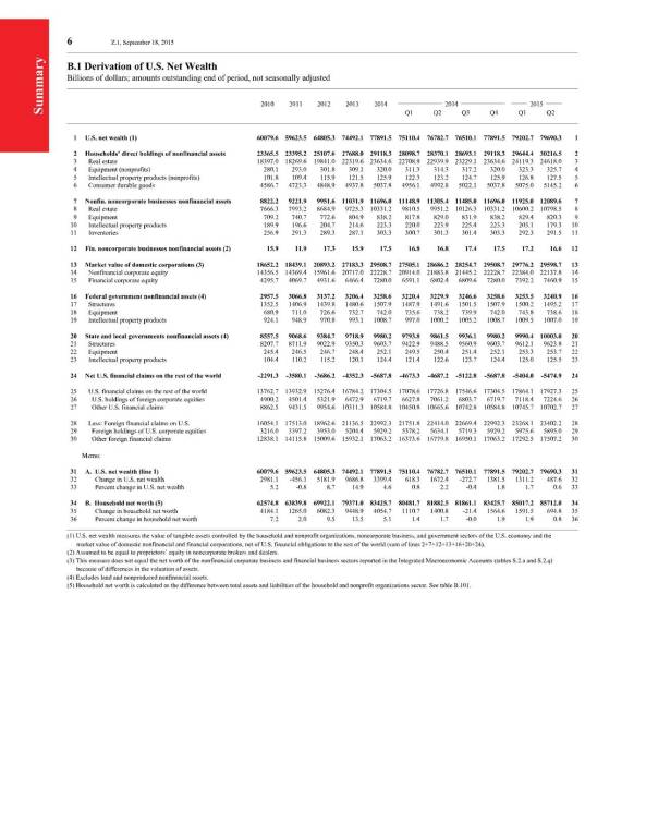
The latest release of the Federal Reserve Statistical Release Z.1, Financial Accounts of the United States – Flow of Funds, Balance Sheets and Integrated Macroeconomic Accounts or just “flow of funds” has a new table B.1: Derivation of U.S. Net Wealth.

According to the release:

A new table on the derivation of U.S. net wealth (table B.1) has been added to the summary section of the “Financial Accounts.” The calculation of U.S. net wealth includes the value of nonfinancial assets (real estate, equipment, intellectual property products, consumer durables, and inventories) held by households and nonprofit organizations and noncorporate businesses. For the federal government and state and local governments sectors, only structures, equipment, and intellectual property products are included; values for land and nonproduced nonfinancial assets are not available. The measure of U.S. net wealth also includes the market value of domestic nonfinancial and financial corporations, and is adjusted to reflect net U.S. financial claims on the rest of the world. This definition of U.S. net wealth differs from the sum of the net worth of sectors shown in the Integrated Macroeconomic Accounts (IMA). A forthcoming FEDS Note will provide additional information.
United States Net Worth

click to expand, and click again to zoom

According to it, the United States net wealth was $79.69 trillion.

It’s important to understand how this is reached. Normally we divide the world in various sectors: households, production firms, the financial sector, government and the rest of the world. In real life one adds more nuances to all this. So for example, in the table above, we have a sector “non-financial non-corporate businesses”.

Now, there are two types of assets: non-financial assets and financial assets. Non-financial assets are things such as houses, machines and so on. Financial assets are things such as currency notes, bonds, equity securities and so on.

In the system of national accounts (e.g., the 2008 SNA), all financial assets have a counterpart liability. So financial assets = liabilities for the world as a whole. It’s of course not true for a nation because assets and liabilities between residents and non-residents do not cancel out.

There is one complication, however: equity securities. The 2008 SNA treats equity securities as liabilities of corporations, just like debt securities. This is despite the fact that a company isn’t bound by law to pay dividends to holders of equity, unlike the case for debt securities or loans (for which interest is needed to be paid periodically and also the principal upon maturity).

All economic units have a net worth. This is the difference between assets and liabilities. So,

Assets = Liabilities + Net Worth.

Since equities are treated as liabilities in the 2008 SNA, the net worth of firms can in fact turn negative. This might happen if the price of equities is high.

So it is easy to derive the net worth of a nation. Resident economic units’ liabilities held by resident economic units cancel out and one is left with non-resident units’ liabilities to residents (i.e., resident units’ assets “held abroad”) and residents’ liabilities to non-residents.  This is the net international investment position.

So, as per the 2008 SNA (and the Balance of Payments Manual, 6th Edition),

Net Worth of a nation = Non-financial assets held by residents + Net International Investment Position

The Federal Reserve however does not do the same for flow of funds. It does not treat equities as liabilities.

But one has to be careful about double counting. It’s easy to sum up non-financial assets of all economic units, such as as done by the SNA. But in the flow of funds, with the special treatment on equities, we shouldn’t use corporate businesses’ non-financial assets. If you read the explanation and see the table B.1 carefully, corporate businesses’ assets have not been added, only “non-corporate businesses'” non-financial assets have been added. Since equities are not treated as liabilities in the sense of debt securities, the market value of corporations is needed to be added. This is line 13 in Table B.1.

There is one complication however. Even though equities is not treated as liabilities, that held by foreigners is treated as liabilities. Otherwise, one can have a source of inconsistency. Suppose equities held by a non-resident economic units is not treated as liabilities. Suppose foreigners sell $1bn of equities and purchase T-bills with that. This will mean that the net wealth reduces. Which doesn’t make sense. Hence, one is forced to treat foreigners’ equity holdings as liabilities. So the foreign aspect of the whole calculation is the same as as done in the SNA and one needs to include the net international investment position of the United States which is line 24. (minus $5.47 trillion).

So that basically summarizes the calculation of the United States net wealth as per the Federal Reserve flow of funds report.

How does this compare with the SNA measurement? Some tables in the report are only updated to 2014. So let’s use those numbers.

Flow of funds’ net wealth for 2014 = $77.89 tn (Table B.1, line 1).

Now, go to Table S.2.a. These tables use SNA definitions. Add lines 76-81.

This gives us a value of $87.34 trillion.

However the Z.1 report has an error in the way SNA/IMA way of calculating net worth. Line 77 in Table S.2.a is incorrect. There’s double counting. It uses the SNA/IMA concept of net worth but instead calculates it using the FoF concept. One should subtract line 29 in table B.101 which is $10.04 trillion. Hence the US net worth in the SNA definition is $87.34 trillion minus $10.04 trillion which is $77.30 trillion.

So in short, the net worth of the United States as per the flow of funds definition at the end of 2014 was $77.89 trillion and according to the SNA/IMA it was $77.30 trillion.

What does all this mean? Hmm. Not to easy to answer, except saying that familiarity with the system of measurement helps in understanding how the economy works. Which measurement is better – the new table B.1 or S.2.a? Doesn’t matter.

I am thankful to commenters in this blog post by Steve Randy Waldman, especially JKH and Marko.

Part 2 here United States’ Net Wealth, Part 2
Credit And Economic Growth

In a new column for Bloomberg, Noah Smith questions the intuition that credit fuels economic growth.

click to view on Twitter

He says:

It seems like the only people who don’t instinctively believe in credit-fueled growth are academic economists.

The academics have good reason for being skeptical.

His reason (in short) is the following:

It’s pretty obvious how credit drives my personal household consumption. If I borrow, I can get a nice big TV and a new car, but eventually I’ll have to skimp to pay it back. In a way, the consumption-fueled borrowing binge is an illusion of wealth — after all, borrowing doesn’t increase my salary. Pleasure today means pain tomorrow.

Notice how Smith’s argument uses a lot of national accounting and flow of funds concepts: consumption, borrowing, wealth, repayment (of loans) and so on. The interesting thing is that one can use the system of national accounts and flow of funds to create models which show precisely the opposite of what Smith is saying. The best place obviously to look out for is the book Monetary Economics: An Integrated Approach to Credit, Money, Income, Production and Wealth by Wynne Godley and Marc Lavoie which has models called stock-flow consistent models or SFC models. It is however difficult to write down a simple SFC model in a blog post, so I will try to highlight how it works in words but refer the reader to these models.

Here’s how in a simple model:

  1. Consumers decide to borrow more and banks respond by granting them loans.
  2. Consumers spend the funds received on consumption goods.
  3. Since loans make deposits, it’s not as if someone forgoes consumption to lend as neoclassical textbooks say.
  4. Firms see their inventories go down and respond by increasing their inventories by producing more.
  5. For producing more, firms hire more labour and pay salary/compensation.
  6. People newly employed spend their income and there’s further rise in production as firms produce more when seeing a higher demand for their products.
  7. Higher production leads to a rise in productivity and wages/household incomes of the already employed rise in response (although not necessarily the case).

So we have a higher output than what we started with and higher national income.

One can take several issues with this and this is one reasons models are really helpful and pinpoint what’s going on. This is the reason I referred to the book by Godley and Lavoie above. So for example, one can ask: what if the rise in the national income and output is just a rise in the nominal value but that it’s possible that prices have changed and that the real output hasn’t changed. This of course needs a model of prices and inflation but a familiarity with stock-flow consistent models will make you realize that it is an extreme assumption to think that the real output hasn’t risen in the sequence of events highlighted above.

The second thing is the above “model” in words had just banks lending to households whereas in the real world, credit (as in any credit, such as firms borrowing) is via credit markets of which banks are only one part. This issue is not so simple to argue out, but it can be shown that it really doesn’t matter (in the first approximation). I do not know how to quickly argue it out in short here but will leave that for now.

Of course the above model can be misleading. For example, if households take a lot of debt, debt repayment burden will hit and cause a slowdown as households’ consumption will drop and this may lead to an economic slowdown. This point may look similar to what Noah Smith is saying, but that is not the case. One can imagine an economy starting with a GDP of 100 and growing to 120 in some time period and then slowing down to 118 because of the debt burden. Also the above model was implicitly a pure private sector model and in general one has both the government and the overseas sector adding more complications. Again more reasons why having a proper mathematical model for such things is important.

Another critique of Smith (in my mini-exchange of tweets with him on Twitter) was that SFC models do have behavioural assumptions. I agree, but my point was that there’s no reason to dismiss the argument “credit fuels growth” by purely theoretical arguments. If at all, the system of national income and flow of funds make it more convincing that credit is important.

Of course none of this means that policies should be promoted to ease credit conditions always and try to create a boom and what Smith says is somewhat true – there can be pain later, so it is important to consider fiscal policy, balance of payments and so on but the story told here is quite different from the one told by Noah Smith.

Profits And Borrowing

I think Marshall Auerback is seriously mixing up different parts of the flow of funds accounts of an economy. He is heteredox, so it will be good if he gets these things right.

In his latest, he asks Why Are US Corporations Borrowing So Much If Profits Are At A Record Percentage Of GDP? (original link no longer works, replaced by web.archive.org alternative), i.e., the reported profits seems contradictory to the fact that borrowing is rising. As mentioned in my recent blog post Massive Overstatement Of Profits?, Auerback attributes it to firms cooking the books. In his latest, he says:

 … debt is once again rising relative to GDP.  That shouldn’t be happening if corporate savings (profits) are booming.

Funnily, his question precisely has the answer: because profits are rising, so has liabilities of U.S. firms, because increased profits has led them to increase investment. This can easily be shown via a few national accounts/flow of funds identities. For the nonfinancial production firms sector, we have:

Net Lending = Undistributed Profits − Investment

Profits is undistributed profits plus dividends, and net lending is net acquisition of financial assets less net incurrence of liabilities,

Net Lending = NAFA − NIL

so,

NIL = Investment − Profits + Dividends + NAFA

where NIL and NAFA are firms’ net incurrence of liabilities and net acquisition of financial assets, respectively in the language of the flow of funds or the system of national accounts such as the 2008 SNA.

This suggests that if profits rise, firms may incur less liabilities but assuming other things in the equation stay the same. But if other things are themselves changing — such as if investment is rising, profits can rise simultaneously with rising liabilities. It is slightly paradoxical at first but CFOs generally know that firms’ borrowing requirement may rise when it is growing fast and the same is possible even if firms are taken as a whole. Firms may also buy back shares by borrowing from banks and this adds more interesting things to the story.

Of course, it is possible that the rising debt may move into an unsustainable territory but this story is a bit different than cooking the books interpretation of Auerback.