Tag Archives: marc lavoie

Open Mouth Operations

In the previous post Is Paul Krugman A Verticalist?, I discussed the confusions economists and market commentators have on open market operations. Even top economists such as Krugman suffer from confusions on central banking and monetary matters.

I also mentioned the work of Alfred Eichner on bringing out more clarity on the defensive nature of open market operations. Let’s look at these matters more closely.

Before this let’s look at what people in general think. Most people think of open market operations as some kind of extra activity on the part of the central bank in collaboration with the bureau of engraving and printing and think of it as operational implementation of Milton Friedman’s helicopter drops! So when a central bank such as the Federal Reserve changes its target on interest rates – such as lowering the “Fed Funds target rate”, people start commenting as if the Federal Reserve is undertaking a mystical operation.

This is Monetarist or Verticalist intuition. It is easy to show that open market operations have nothing to do with fiscal policy and as we saw in the previous blog – very little with monetary policy itself. The open market operation of the central bank is not an income/expenditure flow such as government expenditure flows or tax flows and the former does not affect the net worth of the change the net worth of either the domestic private or the foreign sector. Hence it is hardly fiscal. Yet commentators and economists keep arguing that the central bank is “injecting money” into the economy!

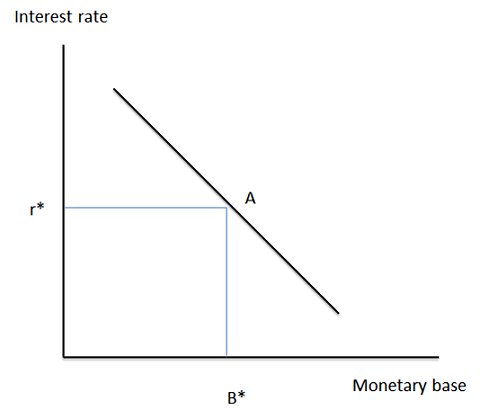
Even Paul Krugman erred on some of these matters and was shown how to do good economics by Scott Fullwiler in his post Krugman’s Flashing Neon Sign. Missing everything Fullwiler was saying, Krugman wrote another post A Teachable Money Moment which has the following diagram:

Below we will see how Krugman’s Neoclassical/New Keynesian (whichever) intuition is flawed.

Setting Interest Rates

These matters (the public understanding) have become worse ever since the Federal Reserve and other central banks around the world started purchasing government debt in the open markets on a large scale – in programs called Large Scale Asset Purchases (also called “QE”). In the following I will consider cases when there is no “asset purchase program” by the central bank and tackle this issue later in another post.

A simple case to highlight how a central bank defends an interest rate (as opposed to changing it) is considering the corridor system. There target for overnight rates is usually at the midpoint of this “corridor”. At the lower end of the corridor banks get paid interest on their settlement balances they keep at the central bank while at the upper end it is the rate at which the central bank lends.

Because banks settle among each other on the books of the central bank, this gives the latter to fix the short-term rates and indirectly influence long term rates.

Why do banks need to settle with each other?

One of the first economists to understand the endogenous nature of money was Sir Dennis Holme Roberston who used to work for the Bank of England. In 1922, he wrote a nice book simply titled Money.

 From page 52:

. . . If A who banks at bank X pays a cheque for £10 to B who banks at bank Y, then Bank Y, when it gets the cheque from B, will present it for payment to Bank X: and bank X will meet its obligation by drawing a cheque for £10 on its chequery at the Bank of England. As a matter of fact, the stream of transactions of this nature between big banks is so large and steady in all directions that the banks are enabled to cancel most of them out by an institution called the clearing-house:  but the existence of these chequeries at the Bank of England facilitates the payment of any balance which it may not be possible at the moment to deal with in this way …

Because banks finally settle at the central bank finally, central banks have learned since their creation that they can set interest rates. This is strongest at the short end of the “yield curve” but directly or indirectly central banks also influence long term rates.

At the end of each day, some banks will be left with excess of settlement balances (if they see more inflows than outflows) and some banks will face the opposite situation. Because they need to satisfy a reserve requirement at the central bank (which can be zero as well), some banks would need to borrow funds from others. Borrowing means paying back with interest and this is where the central bank’s ability to target rates comes enters the picture.

For suppose some bank X needs funds and other banks wish to lend bank X at a very high interest rate. In this scenario bank X can simply borrow from the central bank, while other banks who demanded higher interest will see themselves with excess settlement balances earning less than the target rate. So it would have been better for the latter to have lent than keep excess balances. (Of course the qualifier is that these things are valid under scenarios when there is less stress on the financial system). Also with the same logic, the rate at which banks lend each other will not fall below the corridor because it will be foolish of a bank to have lent settlement balances to another bank when it could have earned higher by just keeping excess settlement balances at the central bank.

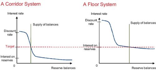
Here is a diagram from the post Corridors And Floors In Monetary Policy from FRBNY’s blog which explains central bank’s operations:

The other system as per this post is the floor system – in which the central bank’s target is the interest paid on settlement balances itself, rather than the midpoint of any corridor. This is what has been followed by the US Federal Reserve in recent times.

Back to the corridor system, an important question arises. Hopefully the reader is convinced that the overnight rate at which banks lend each other is between the corridor. However it is still unclear how and why the central bank can keep it at the midpoint.

If the central bank and the bankers understand the system well, it is possible for the central bank to be quite perfect in this. This happens for example in the case of Canada, where the bank is quite accurate in its objective.

The reason is that the central bank can easily add and subtract settlement balances by various means.

Take an example. Suppose the interest on reserves is 2.25%, the target is 3.00% and the discount rate – the rate at which the central bank lends overnight – 3.75%. If the central bank observes that banks are lending each other at 3.25% – slightly away from the target of 3.00%, it can simply create excess balances. Among the many ways, there are two –

  1. purchase/sale of government securities and/or repurchase/reverse repurchase agreements.
  2. shifts of government deposits from the central bank account into the Treasury’s account at banks or the opposite.

So the central bank knows how the curve in the figure above looks like and adds/subtracts settlement balances by the above methods (mainly). So banks are lending each other at 3.25%, the central bank will add settlement balances; if they are lending each other at 2.75% – the central bank will drain settlement balances.

More generally the “threat” by the central bank is reasonably sufficient to make banks lend at the target!

Open Mouth Operations

Let us suppose the central bank had been targeting 3.00% for three months now and decides to decrease rates.

What does it do?

Almost nothing!

The announcement itself will make banks gravitate toward the new target!

In his paper Monetary Base Endogeneity And The New Features Of The Asset-Based Canadian And American Monetary Systems, Marc Lavoie says:

When they [central banks] are not accommodating—that is, when they are pursuing “dynamic” operations as Victoria Chick (1977, p. 89) calls them—central banks will increase (or decrease) interest rates. As shown above, to do so, they now need to simply announce a new higher target overnight rate. The actual overnight rate will gravitate toward this new anchor within the day of the announcement. No open-market operation and no change whatsoever in the supply of high-powered money are required.

Hence the term “open mouth operations” which was coined by Julian Wright and Greame Guthrie in their paper Market-Implemented Monetary Policy with Open Mouth Operations.

Open Market Operations

The above paper by Marc Lavoie is an excellent source for open market operations and looking at central banking from an endogenous money viewpoint.

I mentioned in the previous post that the open market operations are defensive. In my analysis in this post till now, I ignored the factors which cause settlement balances of the banking sector as a whole to change. Let us bring in this complication.

Apart from banks, the Treasury – the domestic government’s fiscal arm – and other institutions such as foreign central banks, governments and international official institutions (such as the IMF) also keep an account at the (domestic) central bank. When these institutions transact, there is an addition/subtraction of banks’ settlement balances at the central banks.

Here’s one example. Suppose the Treasury transfers funds of $1m to a contractor for settlement of a project done by the latter. When the funds are transferred, the contractor’s bank account increases by $1m and the bank in which he banks sees its deposits and settlement balances rise by $1m while the central bank will reduce the Treasury’s deposits by $1m.

This may lead to a deviation of banks’ lending rate to each other and the central bank needs to drain reserves. The central bank can achieve this by shifting government funds at a bank into the central bank account. If the central bank transfers $1m of funds, banks’ deposits and settlement balances reduce by $1m and the Treasury’s account at the central bank will increase by $1m.

This is not an “open market operation” but another way of adding/draining reserves. In general, depending on institutional setups, the central bank may also do purchase/sale of government securities and/or repurchase agreements.

But this has nothing to do with policy itself – rather it is to maintain status quo. (Of course “large scale asset purchases” is a slightly different matter – first one needs to understand the corridor system).

In other words, this is a defensive behaviour on part of the central bank.

Alfred Eichner

In the previous post and in Alfred Eichner And Federal Reserve Operating Procedures, I mentioned about the contribution of Eichner. In an essay in honour, Alfred Eichner, Post Keynesians, And Money’s Endogeneity – Filling In The Horizontalist Black Box, (from the book Money And Macrodynamics – Alfred Eichner And Post-Keynesian Economics) Louis-Philippe Rochon says:

For Eichner, the overall or “primary objective [of the central bank], in conducting its open market operations, is to ensure the liquidity of the banking system,” which applies to either the accommodating or defensive roles. In either case, Eichner argues that “the Fed’s open market operations are largely an endogenous response to . . . the need both to offset the flows into and out of the domestic monetary-financial system and to provide banks with the reserves they require”; that is, resulting from the demand for money and the demand for credit respectively (1987, 847, 851).

And while the accommodating argument has been debated at length by post-Keynesians, the defensive role has been virtually ignored and only recently rediscovered (see Rochon 1999). Yet it is certainly Eichner’s greatest contribution to the post-Keynesian theory of endogenous money. . .

. . . The “defensive” behavior is defined by Eichner as the “component of the Fed’s open market operations [consisting] of buying or selling government securities so that, on net balance, it offsets these flows into or out of the monetary-financial system,” leaving the overall amount of reserves unchanged. This is the result of changes in portfolio decisions and increases or decreases in bank (demand) deposits. As a result of an increase in the nonbank’s desire to hold currency, for instance, “in order to maintain bank reserves at the same level, the Fed will need to purchase in the open market government securities equal in value to whatever additional currency the nonbank public has decided to hold” (Eichner 1987, 847).

In making the distinction between temporary and permanent open market operations, Rochon also quotes Scott Fullwiler:

Outright or permanent open market operations are primarily undertaken to offset the drain to Fed balances due to currency withdrawals by bank depositors. . . . Temporary open market operations are aimed at keeping the federal funds rate at its target on average through temporary additions to or subtractions from the quantity of Fed balances. Temporary operations attempt to offset changes in Fed balances due to daily or otherwise temporary fluctuations in the Treasury’s account, float, currency, and other parts of the Fed’s balance sheet, in as much as is necessary to meet bank’s demand for Fed balances. (2003, 857)

Paul Krugman

All this is completely opposite of Paul Krugman’s position that

. . . And currency is in limited supply — with the limit set by Fed decisions.

And Krugman’s mistake is not minor – it seems he is completely unaware of the huge difference money endogeneity makes.

So what is the difference between Krugman’s diagram and the one from FRBNY blog – even though they look similar? The difference is that the latter is descriptive of behaviour when policy is unchanged and is useful for describing open market operations etc while Krugman uses the same to describe policy changes – which in reality happen via open mouth operations. Paul Krugman confuses open market operations and open mouth operations. So much for a “teachable money moment”.

Krugman also shows his Monetarist intuition by claiming:

And which point on that curve it chooses has large implications for the economy as a whole. In particular, the Fed can always choke off a private-sector credit boom by moving up and to the left.

implying that the central bank in reality controls the monetary base and thence the money stock.

Some Post Keynesians argued since long ago that the central bank cannot control the money stock:

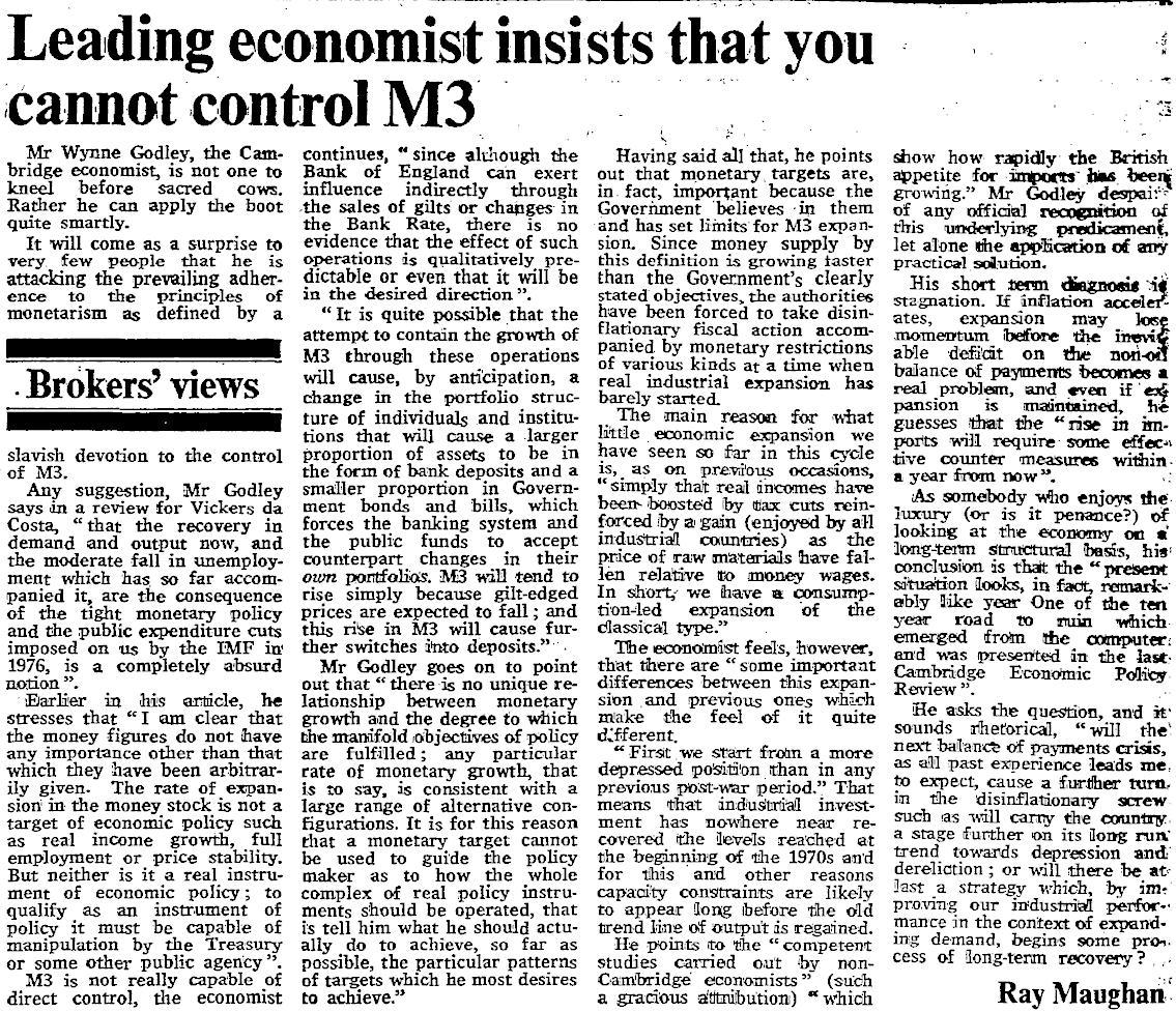
Here’s on Wynne Godley from from The Times, 16 June 1978:

(click to enlarge)

Is Paul Krugman A Verticalist?

24 years back, Basil Moore wrote a book Horizontalists And Verticalists: The Macroeconomics Of Credit Money (Cambridge University Press, 1988) which begins like this:

The central message of this book is that members of the economics profession, all the way from professors to students, are currently operating with a basically incorrect paradigm of the way modern banking systems operate and of the causal connection between wages, prices, on the one hand, and monetary developments, on the other. Currently, the standard paradigm, especially among economists in the United States, treats the central bank as determining the money base and thence the money stock. The growth of the money supply is held to be the main force determining the rate of growth of money income, wages, and prices.

… This book argues that the above order of causation should be reversed. Changes in wages and employment largely determine the demand for bank loans, which in turn determine the rate of growth of the money stock. Central banks have no alternative but to accept this course of events, their only option being to vary the short-term rate of interest at which they supply liquidity to the banking system on demand. Commercial banks are now in a position to supply whatever volume of credit to the economy their borrowers demand.

The book built on his own work and that of Nicholas Kaldor and Marc Lavoie among others goes on to describe the banking system, horizontalism and endogenous money. Money is credit-led and demand-determined was his message. Economists believing in the “incorrect paradigm” are Verticalists in Moore’s terminology.

Paul Krugman whom Post Keynesian have more respect than other mainstream economists probably disappointed them when he was arguing with Steve Keen in a 3-post blog series. Arguing like a Verticalist, Krugman claims (among other Verticalist claims) in his post Banking Mysticism, Continued:

… And currency is in limited supply — with the limit set by Fed decisions. So there is in fact no automatic process by which an increase in bank loans produces a sufficient rise in deposits to back those loans, and a key limiting factor in the size of bank balance sheets is the amount of monetary base the Fed creates — even if banks hold no reserves.

The Defensive Nature Of Open Market Operations

The reason there is widespread misunderstanding of what the central bank does is because it carries out open market operations where it buys or sells government securities or does repurchase agreements. The orthodox view is that the central bank is acting the way it is to increase or decrease the amount of banks’ settlement balances and this affects the money supply – allowing banks to expand lending or leading them to contract – and thence the whole economy. The view is that the central bank has a direct control these operations and are purely volitional.

This is an incorrect view because no central bank claims to be “controlling” the money stock.

If money is truly endogenous, the question is why the central bank does these operations often. The reason is that operations of the central bank are defensive. 

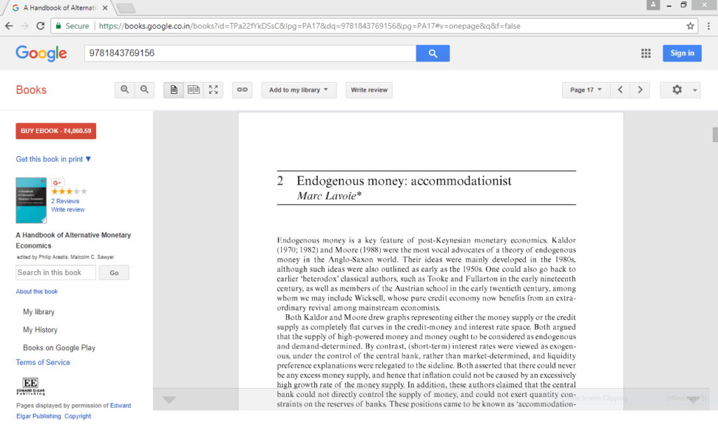
In his article Endogenous Money: Accomodationist, Marc Lavoie argues:

Some post-Keynesians have pointed out long ago that open market operations had little or nothing to do with monetary policy.

For instance, It is usually assumed that a change in the Fed’s holdings of government securities will lead to a change, with the same sign attached, in the reserves of the commercial banking system. It was the failure to observe this relationship empirically which led us, in constructing the monetary financial block of our model, to try to find some other way of representing the effect of the Fed’s open market operations on the banking system. (Eichner, 1986, p. 100)

That other way is that ‘the Fed’s purchases or sales of government securities are intended primarily to offset the flows into or out of the domestic monetary-financial system’ (Eichner, 1987, p. 849).

So the central bank purchases government bonds and/or does repos to neutralize the effects of transactions which change the settlement balances. One example is the flow of funds into and out of the government’s account at the central bank. Another is the demand for currency notes by banks to satisfy their customers’ needs. The central bank has no choice but to provide these notes.

Here’s a preview via Google Books:

click to view on Google Books

Also see this post Alfred Eichner And The Federal Reserve Operating Procedures.

Krugman is partly right when he says, “Banks are important, but they don’t take us into an alternative economic universe.” However he fails to see that money is endogenous and the way the banking system works show this endogeneity.

Of course, Steve Keen has issues with his models and accounting with which Krugman has troubles. Keen defines aggregate demand to be gdp plus “change in debt”. As much weird this definition is, it is double counting when investment expenditure is financed by borrowing rather than internal sources of funds. Also, if a person sells a home to another person who has financed this purchase by borrowing and the former does not make expenditure from this income, this does not increase aggregate demand – a point raised by Marc Lavoie here (h/t “Circuit” from Fictional Reserve Barking). But as per Keen’s definition it does. In his first post, Krugman seems to say the same thing as Lavoie – but in a roundabout way.

The resulting debate has however highlighted the Verticalist intuition of Krugman!

Income And Expenditure Flows And Financing Flows

In the previous two posts, I went into a description of the transactions flow matrix and the balance sheet matrix as tools for an analytic study of a dynamical study of an economy.

During an accounting period, sectors in an economy are making all kinds of transactions. These can be divided into two kinds:

  1. Income and Expenditure Flows
  2. Financing Flows

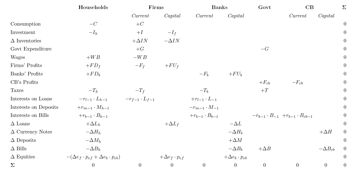
Let’s have the transactions flow matrix as ready reference for the discussion below.

(Click for a nicer view in a new tab)

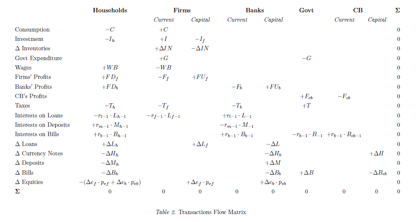
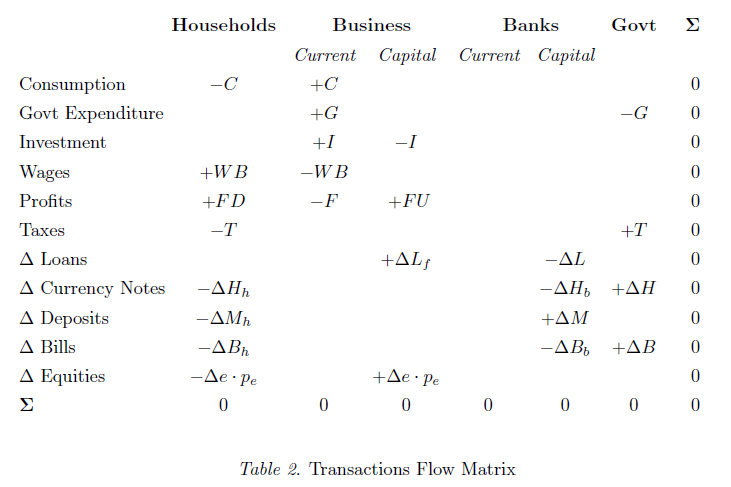
The matrix can easily be split into two – on top we have rows such as consumption, government expenditure and so on and in the bottom, we have items which have a “Δ” such as “Δ Loans” or “change in loans”. We shall call the former income and expenditure flows and the latter financing flows.

To get a better grip on the concept, let us describe household behaviour in an economy. Households receive wages (+WB) and dividends from production firms (called “firms” in the table) and banks (+FD_{f} and +FD_{b}) respectively) on their holdings of stock market equities. They also receive interest income from their bank deposits and government bills. These are sources of households’ income. While receiving income, they are paying taxes and consuming a part of their income (and wealth). They may also make other expenditure such as buying a house or a car. We call these income and expenditure flows.

Due to these decisions, they are either left with a surplus of funds or a deficit. Since we have clubbed all households into one sector, it is possible that some households are left with a surplus of funds and others are in deficit. Those who are in surplus, will allocate their funds into deposits, government bills and equities of production firms and banks. Those who are in deficit, will need funds and finance this by borrowing from the banking system. In addition, they may finance it by selling their existing holding of deposits, bills and equities. The rows with a “Δ” in the bottom part of transactions flow matrix capture these transactions. These flows will be called financing flows.

How do banks provide credit to households? Remember “loans make deposits”. See this thread Horizontalism for more on this.

This can be seen easily with the help of the transactions flow matrix!

The two tables are some modified version of tables from the book Monetary Economics by Wynne Godley and Marc Lavoie.

It is useful to define the flows NAFA, NIL and NL – Net Accumulation of Financial Assets, Net Incurrence of Liabilities and Net Lending, respectively.

If households’ income is higher than expenditure, they are net lenders to the rest of the world. The difference between income and expenditure is called Net Lending. If it is the other way around, they are net borrowers. We can use net borrowing or simply say that net lending is negative. Now, it’s possible and typically the case that if households are acquiring financial assets and incurring liabilities. So if their net lending is $10, it is possible they acquire financial assets worth $15 and borrow $5.

So the the identity relating the three flows is:

NL = NAFA – NIL

I have an example on this toward the end of this post.

I have kept the phrase “net” loosely defined, because it can be used in two senses. Also, some authors use NAFA when they actually mean NL – because previous system of accounts used this terminology as clarified by Claudio Dos Santos. I prefer old NAFA over NL, because it is suggestive of a dynamic, though the example at the end uses the 2008 SNA terminology.

While households acquire financial assets and incur liabilities, their balance sheets are changing. At the same time, they also see holding gains or losses in their portfolio of assets. What was still missing was a full integration matrix but that will be a topic for a post later. Since, it is important however, let me write a brief mnemonic:

Closing Stocks = Opening Stocks + Flows + Revaluations

where revaluations denotes holding gains or losses.

This is needed for all assets and liabilities and for all sectors and hence we need a full matrix.

We will discuss more on the behaviour of banks (and the financial system) and production firms some other time but let us briefly look at the government’s finances.

As we saw in the post Sources And Uses Of Funds, government’s expenditure is use of funds and the sources for funds is taxes, the central bank’s profits, and issue of bills (and bonds). Unlike households, however, the government is in a supreme position in the process of “money creation”. Except with notable exceptions such as in the Euro Area, the government has the power to make a draft at the central bank under extreme emergency, though ordinarily it is restricted. Wynne Godley and Francis Cripps described it as follows in their 1983 book Macroeconomics:

Our closed economy has a ‘central bank’ with two principle functions – to manage the government’s debt and to administer monetary policy. [Footnote: The central bank has to fund the government’s operations but this in itself presents no problems. Government cheques are universally accepted. When deposited with commercial banks the cheque become ‘reserve assets’ in the first instance; banks may immediately get rid of excess reserve assets by buying bonds.]. The only instrument of monetary policy available to the central bank in our simple system is the buying and selling of government bonds in the bond market. These operations are called open market operations. We assume that the central bank does not have the right to directly intervene directly in the affairs of commercial banks (e.g., to prescribe interest rates or quantitative lending limits) or to change the 10% minimum reserve requirement. But the central bank is in a very strong position in the bond market since it can sell or buy back bonds virtually without limit. This gives it the power, if it chooses, to fix bond prices and yields unilaterally at any level [Footnote: But speculation based on expectations of future yields may oblige the central bank to deal on a very large scale to achieve this objective.] and thereby (as we shall soon see) determine the general level of interest rates in the commercial banking system.

Given such powers, we can assume in many descriptions that the government’s expenditure and the tax rate is exogenous. However, many times, there are many constraints such as price and wage rises, high capacity utilization and low production capacity and also constraints brought about from the external sector due to which fiscal policy has to give in and become endogenous.

While I haven’t introduced open economy macroeconomics in this blog in a stock-flow coherent framework, we can make some general observations:

For a closed economy as a whole, income = expenditure. While it is true for the whole economy (worth stressing again: closed), it is not true for individual sectors. The household sector, for example, typically has its income higher than expenditure. In the last 15-20 years, even this has not been the case. If one sector has it’s income higher than expenditure, some sectors in the rest of the world will have its income lower than its expenditure. Many times, the government has its income lower than expenditure and we see misleading public debates on why the government should aim to achieve a balanced budget. When a sector has its income lesser than expenditure, it’s net lending is negative and hence is a net borrower from the rest of the world. It can finance this by borrowing or sale of assets. A region or a whole nation can have its expenditure higher than income and this is financed by borrowing from the rest of the world. A negative flow of net lending implies a net incurrence of liabilities – thus adding to the stock of net indebtedness which can run into an unsustainable territory. Stock-flow coherent Keynesian models have the power to go beyond short-run Keynesian analysis and study sustainable and unsustainable processes.

In an article Peering Over The Edge Of The Short Period – The Keynesian Roots Of Stock-Flow Consistent Macroeconomic Models, the authors Antonio C. Macedo e Silva and Claudio H. Dos Santos say:

… it is important to have in mind that it is possible to get three kinds of trajectories with SFC models:

  • trajectories toward a sustainable steady state;
  • trajectories toward a steady state over certain limits;
  • explosive trajectories.

The analysis of SFC models’ dynamic trajectories and steady states is useful, first because it makes clear to the analyst whether the regime described in the model is sustainable or whether it leads to some kind of rupture—either because the trajectory is explosive or because it leads to politically unacceptable configurations. In these cases, as Keynes would say in the Tract, the analyst can conclude that something will have to change and even get clues about (i) what will probably change (since the sensitivity of the system dynamics to changes in different behavioural parameters is not the same); and (ii) when this change will occur (since the system may converge or diverge more or less rapidly).

Example

Note that Net Lending is different from “saving”. Say, a household earns $100 in a year (including interest payments and dividends), pays taxes of $20 and consumes $75 and takes a loan of to finance a house purchase near the end of the year whose price is $500. Assume that the Loan-To-Value (LTV) of the loan is 90% – which means he gets a loan of $450 and has to pay the remaining $50 from his pocket to buy the house. (i.e., he is financing the house mainly by borrowing and partly by sale of assets). How does the bank lending – simply by expanding it’s balance sheet (“loans make deposits”). Ignoring, interest and principal payments (which we assume to fall in the next accounting period),

His saving is +$100 – $20 – $75 = +$5.

His Investment is +$500.

His Net Incurrence of Liabilities is +$450.

His Net Accumulation of Financial Assets is +$5 – $50 = – $45.

His Net Lending is = -$45 – (+$450) = -$495 which is Saving net of Investment ($5 minus $500).

This means even though the person has “saved” $5, he has incurred an additional liability of $450 and due to sale of assets worth $45, he is a net borrower of $495 from other sectors (i.e., his net lending is -$495).

Assume he started with a net worth of $200.


Opening Stocks: 2010

$

Assets

200

Nonfinancial Assets
Deposits
Equities

0
30
170

Liabilities and Net Worth

200

Loans
Net Worth

0
200


Now as per our description above, the person has a saving of $5 and he purchases a house worth $500 by taking a loan of $450 and selling assets worth $50. We saw that the person’s Net Accumulation of financial assets is minus $45. How does he allocate this? (Or unallocate $45)? We assume a withdrawal of $10 of deposits and equities worth $35. At the same time, during the period, assume he had a holding gain of $20 in his equities due to a rise in stock markets.

Hence his deposits reduce by $10 from $30 to $20. His holding of equities decreases by $15 (-$35 + $20 = -$15)

How does his end of period balance sheet look like? (We assume as mentioned before that the purchase of the house occurred near the end of the accounting period, so that principal and interest payments complications appear in the next quarter.)


Closing Stocks: 2010

$

Assets

675

Nonfinancial Assets
Deposits
Equities

500
20
155

Liabilities and Net Worth

675

Loans
Net Worth

450
225


Just to check: Saving and capital gains added $5 and $20 to his net worth and hence his net worth increased to $225 from $200.

Of course, from the analysis which was mainly to establish the connections between stocks and flows seems insufficient to address what can go wrong if anything can go wrong. In the above example, the household’s net worth gained even though he was incurring a huge liability. What role does fiscal policy have? The above is not sufficient to answer this. Hence a more behavioural analysis for the whole economy is needed which is what stock-flow consistent modeling is about.

One immediate answer that may satisfy the reader now is that the households’ financial assets versus liabilities has somewhat deteriorated and hence increased his financial fragility. By running a deficit of $495 i.e., 495% of his income, the person and his lender has contributed to risk. Of course, this is just one time for the person – he may be highly creditworthy and his deficit spending is an injection of demand which is good for the whole economy. After all, economies run on credit. While this person is a huge deficit spender, there are other households who are in surplus and this can cancel out. In the last 15 years or so, however (before the financial crisis hit), households (as a sector) in many advanced economies ran deficits of the order of a few percentage of GDP. If the whole household sector continues to be a net borrower for many periods, then this process can turn unsustainable as the financial crisis in the US proved.

Now to the title of the post. Flows such as consumption, taxes, investment are income/expenditure flows. Flows such as “Δ Loans”, “Δ Deposits”, “Δ Equities” are financing flows. Income/expenditure flows affect financing flows which then affect balance sheets, as we see in the example.

Sources And Uses Of Funds

In a recent post, I went into what is called the Transactions Flow Matrix. This is used heavily in Stock-Flow Consistent Modeling of the whole economy. The underlying theme is “everything comes from somewhere and goes somewhere, and there are no black holes”.

I also mentioned about a Balance Sheet Matrix. What is it?

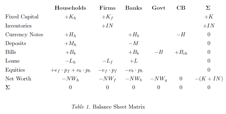
Sectors in an economy have assets and liabilities. Assets can be both financial as well as nonfinancial. Since nonfinancial assets are nobody’s liability, liabilities are financial. Very quickly, a balance sheet matrix is created by assigning a + sign to assets and a (-) sign to liabilities.

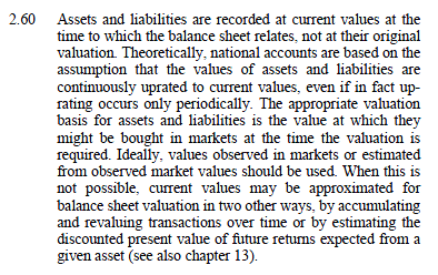
As per the System of National Accounts, all assets and liabilities are to be evaluated at market prices. According to 2008 SNA,

So a corporation or the government may have issued bonds at $100 but since the value fluctuates everyday and even during the day, it is possible that the bond price may reach $103. If it is the last day of the period for which the balance sheet is compiled, then the liability should be entered as $103, not $100.

We will have more to see in another post but let us just have a cursory look at an item called net worth. Since balance sheets should balance, we include this item in liabilities or rather call the right hand side of a balance sheet “Liabilities and Net Worth”. The term Net Worth has an intuitive appeal. If I have assets worth $100 and owe someone (say a bank) $10 and nothing more or less, my net worth is $90.

So let us quickly jump into the balance sheet matrix of a model economy.

In the previous post on the Transactions Flow Matrix, I had amalgamated the sectors Government and Central Bank into one, but now I have separated them so that there is higher clarity.

The reason I am writing this post is to stress the importance of signs. So in the above you will notice that households have a liability of L_{h} and hence appears with a negative sign. We shall see below however, that since loans are a source of funds, it will appear as a positive sign in the transactions flow matrix!

So households hold currency notes, deposits, bills and equities and these have counterpart in some other sector. And this should be the case because every financial asset is someone else’s liability. Also, from the matrix, the sum of net worths of all sectors (for a closed economy, at any rate) is equal to the value of the nonfinancial assets. This result isn’t surprising since financial assets cancel out with their counterpart liabilities.

We now jump to the transactions flow matrix – which I remade and added a lot of complications as compared to the previously related post The Transactions Flow Matrix

(Click to enlarge in a new tab)

These matrices are almost exactly similar to what appears in Wynne Godley and Marc Lavoie’s book Monetary Economics. 

The difference between the two matrices is that the balance sheet matrix records assets and liabilities at the beginning or the end of a period, whereas the transactions flow matrix records transactions during an accounting period.

In the previous post I had briefly stressed the importance of signs but now we have the balance sheet matrix as well ready, let me stress this again using a few lines from G&L’s book on the transaction flow matrix (page 40):

The best way to take it in is by first running down each column to ascertain that it is a comprehensive account of the sources and uses of all flows to and from the sector and then reading across each row to find the counterpart of each transaction by one sector in that of another. Note that all sources of funds in a sectoral account take a plus sign, while the uses of these funds take a minus sign. Any transaction involving an incoming flow, the proceeds of a sale or the receipts of some monetary flow, thus takes a positive sign; a transaction involving an outgoing flow must take a negative sign. Uses of funds, outlays, can be either the purchase of consumption goods or the purchase (or acquisition) of a financial asset. The signs attached to the ‘flow of funds’ entries which appear below the horizontal bold line are strongly counter-intuitive since the acquisition of a financial asset that would add to the existing stock of asset, say, money, by the household sector, is described with a negative sign. But all is made clear so soon as one recalls that this acquisition of money balances constitutes an outgoing transaction flow, that is, a use of funds.

So the government expenditure G has a minus sign because it is a use of funds and its sources are taxes, net issuance of bills and central bank profits.

The sources of funds for the production sector (abbreviated “firms”) is retained earnings (or undistributed profits, called FU), loans from banks and the issuance of equities and also sales (the consumption by households), government purchase of goods and investment itself because producers create tangible capital for themselves as a whole.

Now compare signs in the two matrices – equities are a source of funds for firms and hence has a positive sign in the transactions flow matrix but equities are also liabilities and hence the stock of equities appears with a negative sign in the balance sheet matrix.

Similarly, borrowing via loans are a source of funds for households and hence the positive sign in Table 2 while in Table 1 it appears with a minus sign.

For banks, making loans is a use of funds and taking deposits a source of funds. Hence minus and plus respectively in Table 2.

Also, the equities and loans in Table 2 are flows whereas in Table 1 they are stocks. Hence in Table 2, we have “Δ Loans” or change in loans, whereas in Table 1 its simply “Loans”.

Once we have a beginning of period balance sheet matrix and the transactions flow matrix, how do we construct the end of the period balance sheet matrix? I will leave this question for another post because I will have to introduce capital/holding gains and something called a full integration matrix. Before that I will have another post on real numbers taken from statistical releases to get more a intuitive feel for the balance sheet matrix.

The three matrices (the transactions flow matrix, the balance sheet matrix and the full integration matrix) go into the heart of “how money is created”. For this to be seen in detail, I will have to go into “monetary circuits” using transaction flows and that is the topic of yet another post. If you really understand how loans make deposits, the two tables should set you into a dynamical view of the whole process – a description completely different than the chimerical money multiplier model.

Post Keynesian Markup Pricing

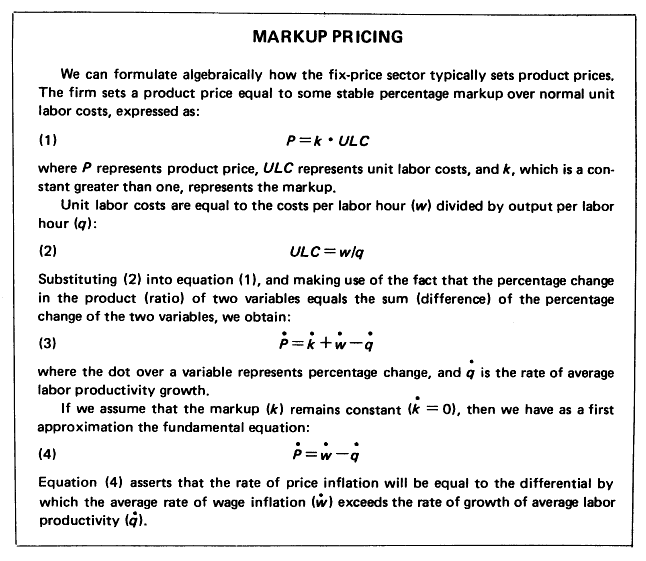
I was collecting some articles by Basil Moore and I found this table from an article In Praise Of Markets – Wage Imitation And Price Stability (unsure as to why the article is titled “praise of markets”). The article appeared in Challenge in 1982.

Post Keynesians adopt Kaleckian theory of pricing. There are two sectors – fix price and flex price.

(The following table is for the fix-price sector).

Of course, this is just a quick and dirty way of getting into Post Keynesian pricing theory which has a rich literature and has obsessed all the leading PKEists for years.

During the 1970s, wages in advanced economies rose due to the rise in the bargaining power of labour unions and this led to a wage-price spiral. As wages increased, firms increased prices in response. This led workers to demand higher wages so as to be compensated for inflation – leading to further price rises. The pricing was also complicated by increase in other costs such as energy prices which led to an increase in markup as well. When firms faced more wage costs, they borrowed more from banks and this led to a huge increase in the money stock. (I am resisting the usage of the  word “supply” for money, as it is misleading). Monetarism came to popularity as the Monetarists led by Milton Friedman were making a lot of noises and saw the relationship and used their political powers to ask central banks to “control” the money stock. When central banks responded saying they do not and cannot control the money stock, Milton Friedman declared them “incompetent”!

Some central banks were forced to bow into political pressures and had to raise short term interest rates (i.e, they still weren’t controlling the money stock, because it cannot be controlled). This had the additional complication that firms’ interest costs (on borrowings) increased and they were forced to increase prices more. In the end, interest rates was raised to such a high level that it led to a huge fall in demand and employment, even though Monetarists’ theories continued claiming that wages will fall and “free markets” will lead to full employment!

During the period (70s/80s), there were also debates about the “velocity of money” – the supposed stability of the relationship of money stock and money income. Some Keynesians try to argue that the relationship is not stable etc. However Marc Lavoie, in an article in response to a comment to his earlier article on endogenous money pointed out:

… The second point I want to raise is the question of the stability of the velocity of money. Gedeon says that an unstable velocity is the typical post Keynesian argument and she goes into a detailed  analysis of a demand for money function that would exhibit this characteristic … I do not think that the stability or instability of the velocity of money is a fundamental question since it ignores the more vital issue of causation. Provided it is recognized that money does not determine income, post Keynesians can feel comfortable  with either stable or unstable velocity.

Monetarism is no longer as popular now as it used to be, but traces can easily be found in most theories of economics such as the “New Consensus”.

S&P Takes Rating Actions On Euro Area Governments

On 5 December 2011, S&P put ratings of EA17 governments on rating watch negative. See my post S&P And EA17 National Governments for link to the S&P report. Today it concluded its review and downgraded several governments.

click to view  the tweet on Twitter

According to the report, which can be obtained from S&P’s Tweet:

We have lowered the long-term ratings on Cyprus, Italy, Portugal, and Spain by two notches; lowered the long-term ratings on Austria, France, Malta, Slovakia, and Slovenia, by one notch; and affirmed the long-term ratings on Belgium, Estonia, Finland, Germany, Ireland, Luxembourg, and the Netherlands. All ratings have been removed from CreditWatch, where they were placed with negative implications on Dec. 5, 2011 (except for Cyprus, which was first placed on CreditWatch on Aug. 12, 2011).

The outlooks on the long-term ratings on Austria, Belgium, Cyprus, Estonia, Finland, France, Ireland, Italy, Luxembourg, Malta, the Netherlands, Portugal, Slovenia, and Spain are negative, indicating that we believe that there is at least a one-in-three chance that the rating will be lowered in 2012 or 2013. The outlook horizon for issuers with investment-grade ratings is up to two years, and for issuers with speculative-grade ratings up to one year. The outlooks on the long-term ratings on Germany and Slovakia are stable.

We assigned recovery ratings of `4′ to both Cyprus and Portugal, in accordance with our practice to assign recovery ratings to issuers rated in the speculative-grade category, indicating an expected recovery of 30%-50% should a default occur in the future.

S&P also cites that “an open and prolonged dispute among European policymakers over the proper approach to address challenges” as one of the reasons to take the rating actions.

How can the Euro Area solve its problems?

One of my favourite papers is A Simple Model Of Three Economies With Two Currencies (link) written by Wynne Godley and Marc Lavoie. The paper was written about 7-8 years back and was published in 2006 in the Cambridge Journal of Economics.

The paper’s abstract:

This paper presents a Keynesian model which describes three countries trading merchandise and financial assets with one another. It is initially assumed that all three countries have independent fiscal policies but that two of the countries share a currency, hence the model can be used to make a preliminary analysis of the conduct of economic policy in ‘the eurozone’ vis-a`-vis the rest of the world—‘the USA’. The main conclusion will be that, if all three countries do indeed operate independent fiscal policies, the system will work under a floating currency regime, but only so long as the European central bank is prepared to modify the structure of its assets by accumulating an ever rising proportion of bills issued by any ‘weak’ euro country.

G&L make an interesting remark about a possible ECB behaviour:

… If the ECB is forbidden from accommodating market-driven changes in the composition of its assets, or if the ECB rules that it will not accumulate additional stocks of securities issued by governments that have excessively large debts according to rating agencies, then fiscal policy in the ‘weak’ countries must be endogenous for stability to prevail, for otherwise it would seem that the only alternative is to let interest rates on euro bills to diverge from country to country in an unsustainable way.

Now this would seem to be a rather dismal state of affairs, from a progressive standpoint. However, it should be noted that balanced fiscal and external positions for all could as well be reached if the euro country benefiting from a (quasi) twin surplus as a result of the negative external shock on the other euro country decided to increase its government expenditures, in an effort to get rid of its budget surplus …

i.e., Euro Area nations with a weak external sector will have to deflate fiscal policy to attempt to keep the external deficit, net indebtedness to the rest of the world and interest rate in check, if surplus nations in the Euro Area do not wish to engage in fiscal expansion. Else, as G&L conclude:

Alternatively, the present structure of the European Union would need to be modified, giving far more spending and taxing power to the European Union Parliament, transforming it into a bona fide federal government that would be able to engage into substantial equalisation payments which would automatically transfer fiscal resources from the more successful to the less successful members of the euro zone. In this manner, the eurozone would be provided with a mechanism that would reduce the present bias towards downward fiscal adjustments of the deficit countries.

In my opinion, this is the only way the Euro Area can come out of the mess because it is the only way the net indebtedness of an EA nation (or a group of nations) can be prevented from exploding relative to its domestic output .

For an earlier take on the Maastricht Treaty by Wynne Godley see the article Maastricht And All That published in the London Review of Books in 1992.

The Transactions Flow Matrix

Why is GDP defined as C+I+G+… and how is it related to national income, expenditure etc and that of each sector of an economy such as that of households?

The following table (redrawn by myself) taken from the book Monetary Economics by Wynne Godley and Marc Lavoie gives an idea on how to go about measuring national income, product etc. The sample chapter (Contents, Chapter 1 & Index) from the publisher’s website has an introduction to the authors’ approach of studying Macroeconomics from a stock-flow consistent approach.

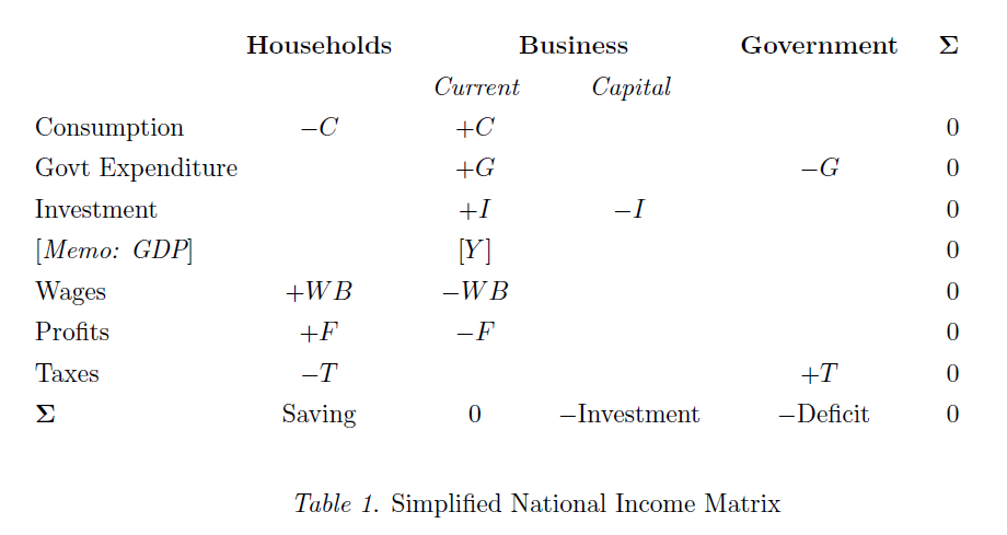
The table describes income and expenditures flows within an economy. Of course, as mentioned this is simplified and complications have to be added one by one. For example, there is no inventories, no external sector and households do not purchase a house etc. However, the above construction shows an easy way of building up and thinking about how funds flow between different ‘sectors’ of an economy. The reader who is new to this way of thinking should pay attention to the signs attached to each entry. For example, households receive wages and it is a source of funds for them and hence the positive sign. When they are consuming, they use funds and hence the first row in the table with the item consumption has a negative sign for households. For businesses, this a source of funds and hence positive. Another item which may be unfamiliar is the capital account of businesses. Firms purchase capital goods for their production and the sale of these goods comes from the same sector and hence one need for this column.

Even at this simplified form, there are a lot which are not known from the above table. What form does saving take? How does the government finance its excess of expenditure over income (i.e., deficit)? How do firms pay for wages and get funds to do the investment etc. To see this, we need a transactions flow matrix which I had discussed previously in my post Financial Crisis And Flow Of Funds from a not-so-pedagogic perspective. It is a foxy trick.

A few things before going into this. First notice that from the matrix,

C + I + G = Y = WB + F

So in our simplified example, gross domestic product is the sum of expenditures on goods and services and at the same time the sum of incomes paid for the production of goods and services.

Second, if you want the actual numbers (for the United States), the place to get this from the Federal Reserve Statistical Release Z.1. In particular, tables F.6 and F.7 and the hyperlink directly takes you to the table.

Back to our question on what form does saving take and how do firms finance their activities etc. Below is the table I made using TeX (and taken from the same book, Chapter 1)

The questions asked also lead us naturally to the introduction of the banking sector and its importance in the process of production, and this sector was missing in Table 1. So we can now clearly see what form saving takes. For households, this is in the form of currency notes, bank deposits, government T-bills and firms’ equities. Apart from various complications added, you may have noticed that profits are assumed to be part distributed and part retained. Firms hence finance investment by retained earnings, loans from banks and by issuance of equities, here. The government finances its deficit (i.e., excess of outlays over receipts) by issuing currency notes and T-bills. We have merged the Central Bank and the Federal Government into one sector “Govt”, for simplicity (which is also the case for Table 1). The behavioural aspects are something different and it should not be assumed that the government can “control” its deficit and that it can choose the proportion of financing in the form of currency notes and bills.

Needless to say, the above transactions flow matrix is a simplified one. For example, you may immediately notice that there is no interest payments on loans and bills yet.

It should be noted here that the entries in the table are flows and hence you may see a lot of Δs. The reader who is relatively new to this should not fail to observe the signs attaching each entry. The negative sign in the entry for deposits for households may be confusing at first, but the self-consistency of the whole construction forces the signs on these entries.

It is worth emphasizing that the fact that all rows and columns sum to zero and this makes the whole construction very appealing. When I was trying to get myself introduced to economics about 3 years back, I browsed around the internet and quickly came across the transactions flow matrix – exactly what I was looking for!

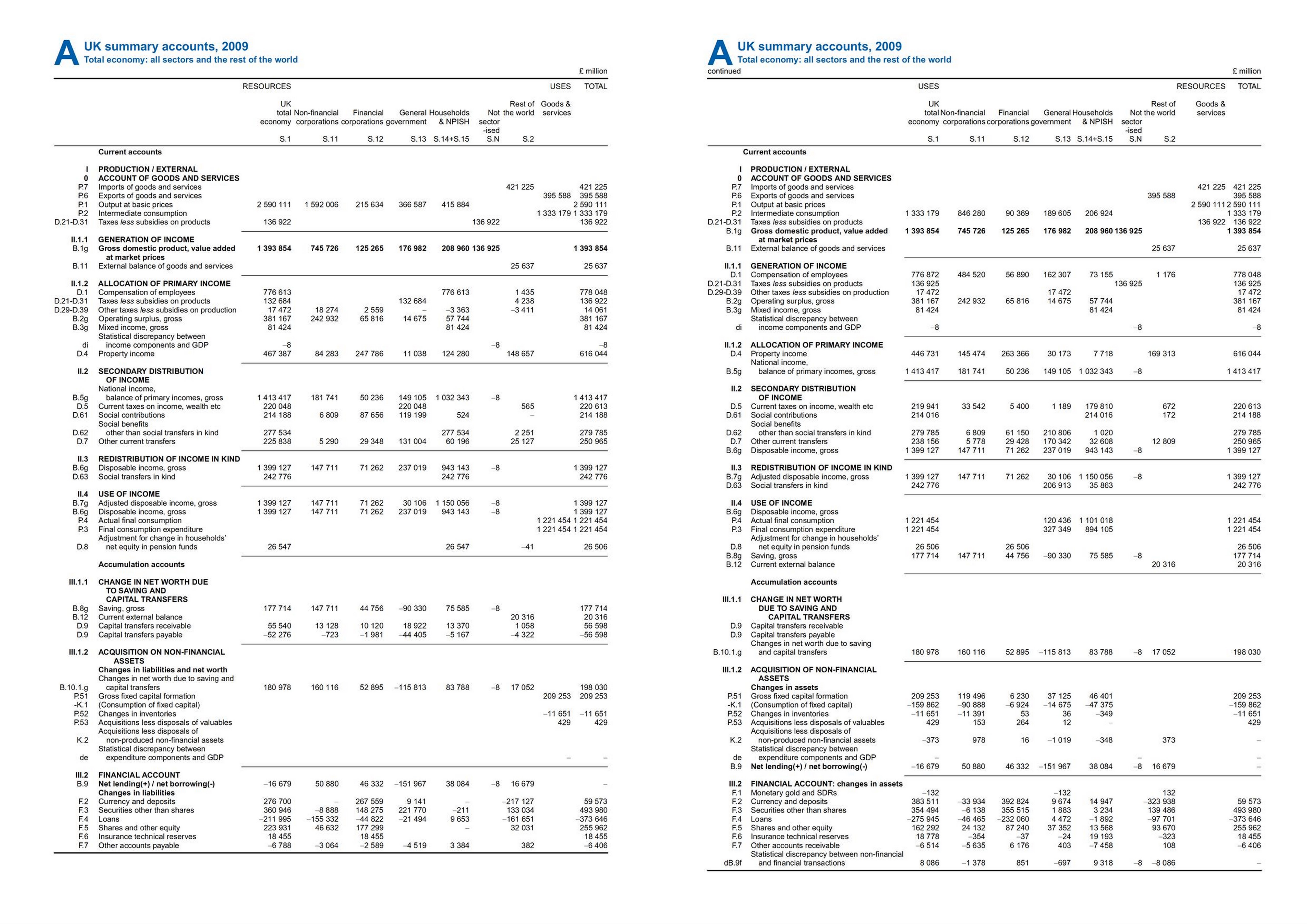
This construction greatly simplifies visualizing flow of funds as compared to the Blue Book way of doing it. The following is the 2008 SNA way of maintaining national accounts and there is some additional effort one needs to visualize this without the usage of a transactions flow matrix!

(click to enlarge)

Books In Honour Of Wynne Godley

There are two new books in honour of Wynne Godley and they are out now

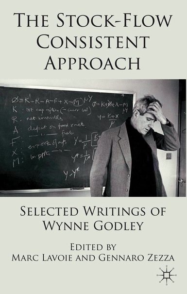
The first one – edited by Marc Lavoie and Gennaro Zezza – has selected articles and papers by Wynne Godley, and carefully chosen.

It’s available at amazon.co.uk, but not yet on amazon.com

Here’s the book’s website on Palgrave Macmillan. The book also contains the full bibliography of Godley’s papers, books, working papers, memoranda (such as to the UK expenditure committee), magazine/newspaper articles, letters to the editor etc.

Here’s a picture I took of Marc at Levy Institute in May when he was deciding on the cover.

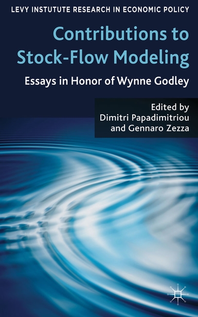
The is second book written in honour of Wynne Godley contains proceeding of the conference held in May at the Levy Institute (the same place the above photograph was taken)

The publisher’s website for the book is here.

Dimitri says:

The death of Wynne Godley silences a forceful and very often critical voice in macroeconomics. Wynne’s own strong view, that although his work was representative of the non-mainstream Keynesian approach to economics and especially economic policy was important nevertheless, has been confirmed time and time again as evidenced in the fortunes of the UK, US and Eurozone economies. His writings, reflecting the sharpness of his mind and intellectual integrity, have had a considerable impact on macroeconomics and have aroused the interest of scholars, economic journalists and policymakers in both mainstream and alternative thought. In a review of Wynne’s last book with Marc Lavoie (2007), Lance Taylor had this to say: ‘Wynne’s important contributions are foxy – brilliant innovations… that feed into the architecture of his models’

I also like Wynne’s stand on the current account imbalance of the United States:

Bibow finds that Godley’s diagnosis of the looming economic and financial difficulties ahead of their occurrence was prescient with regard to US domestic developments – a theme that came up in the chapters by Wray and Galbraith. But Bibow takes issue with Wynne’s assessment of the US external balance being unsustainable. He notes that the US investment position and income flows are more or less in balance and he attributes this phenomenon to the safety of the US Treasury securities and the dollar functioning as the reserve currency.

Dimitri then says

Even if this is so, it cannot continue indefinitely, Wynne would have replied.

The conference page is here

Alfred Eichner And Federal Reserve Operating Procedures

Alfred Eichner was a Post-Keynesian economist known for his text Macrodynamics of Advanced Market Economies published 3 years after his death in 1988. He died at the age of 50 in an accident and at the time he was preparing to include an analysis of open economy macroeconomics in his story of how economies work.

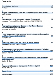
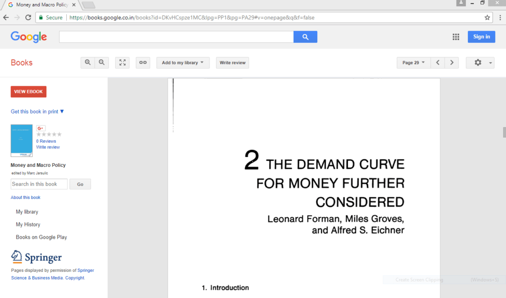
This post is about an article/chapter he wrote (with Leonard Forman and Miles Groves)* in 1984 in a book titled Money And Macro Policy edited by Marc Jarsulic. It is a fantastic book with chapters written by Basil Moore and Marc Lavoie as well on the endogeneity of money. I discussed this previously in my post More On Horizontalism.

Google Books allows a preview of the chapter and embedding it on a webpage and I have done so at the end of this post. If it doesn’t appear properly in your browser, please let me know. Else, like me, you can buy the book 🙂 Of course G-books won’t allow a preview of all pages due to copyright restrictions.

Eichner’s chapter (#2) is titled The Demand Curve For Money Further Considered. 

The authors start off the description with

First, the amount of bank reserves, and thus the monetary base, is not the exogenously determined variable assumed in both orthodox Keynesian and monetarist models but instead depends on the level of nominal income. This is because the central bank, in order to maintain the liquidity of the financial system, is forced to purchase government securities in the open market so as to accommodate, at least in part, the need for additional credit as the pace of economic activity quickens. With the amount of unborrowed bank reserves, and thus the monetary base, to a significant extent endogenously determined, it follows that the money supply is, to no less an extent endogenously determined as well. It is therefore a misspecification to assume that the money stock, or any of its components, is entirely exogenous, subject to the control of the monetary authorities, and then to derive a demand curve for money based on that assumption. In reality, the demand for and supply of “money” are interdependent, with no possibility in practice of being able to distinguish between the two.

Second, it is the demand for credit rather than the demand for money which is the necessary starting point for analyzing the role played by monetary factors in determining the level of real economic activity…

The authors then point out the neutralizing nature of open-market operations of the Fed. Usually this – open market operations – is presented in textbooks and in some old Federal Reserve publications as causing the amount of reserves to rise and allowing banks to increase the supply of reserves. Eichner had earlier worked with data and failed to see open market operations increasing the amount of reserves in practice. He realized that the open market operations neutralize flows:

… Thus, in the face of a fluctuating public demand for currency, flows of gold into and out of the country, variations in the amount of deposits held at the Fed by foreigners and others, changes in the amount of float and fluctuations in the Treasury’s cash holdings, the Fed must engage in open-market operations just to maintain bank reserves at a given level. This is the neutralizing component of a fully accommodating policy, and it is one reason why it is difficult in practice to relate change in bank reserves to open market operations …

What is so nice about the quote above is that Eichner knew exactly what factors affect reserve balances. At the time, “float” may have been more important than it is today. Eichner not only knew that the Treasury’s account at the Fed affects reserve balances but also holdings of other institutions such as foreign central banks – i.e., as a result of “flows of funds into or out of the Federal Reserve System” in his own words. (In the same paragraph from which the quote is taken).

Further the article goes:

An increase in the demand for credit will, to the extent it is satisfied, lead to an increase in bank deposits (especially demand deposits). This is because banks make loans by simply crediting the borrower’s account at the bank with the funds advanced. The increase in deposits will, however, require that banks maintain larger reserves at the Fed. Thus required reserves, ResR, will increase and, unless the Fed acts through the purchase of government securities in the open market to provide banks with the necessary additional reserves, banks will find themselves with insufficient reserves to meet their legal requirements… the Fed is forced to accommodate, at least in part,  whatever demand for credit may manifest itself.

The terminology “accommodating” was later made clear later by Eichner in his book Macrodynamics as operations aimed at pegging the short term interest rate whatever the economic or credit conditions. So when the Fed is not accommodating – in this terminology – it means it is pursuing a policy of raising rates at frequent intervals with an aim to impact credit and aggregate demand.

The Google Books link is embedded below.

click to view on Google Books

Endnote

*Chief Economist and Economic Analyst, respectively at The New York Times at the time of writing.

Z.1, Q3-2011

The Federal Reserve released the Flow of Funds Accounts of the United States today.

The Flow of Funds Accounts provides one of the best snapshot of an economy. In an article appropriately titled ‘No one saw this coming’ – or did they? (see the full paper here), Dirk Bezemer correctly recognizes that the Economics profession’s ignorance of Flow of Funds had a big role to play in its inability to see a crisis coming. Bezemer says

We economists – and the policymakers who rely on us – ignore balance sheets and the flow of funds at our peril.

Of course, as Bezemer points out, there were exceptions. Post Keynesians were always aware of the flow of funds because monetary economy is a natural starting point in their theory. Wynne Godley and Marc Lavoie wrote a book (my favourite!) Monetary Economics: An Integrated Approach To Credit, Money, Income, Production and Wealth, Palgrave Macmillan, 2007, to unify Post Keynesian theory and the flow of funds approach, perhaps improving the presentation of the latter using something called the “transactions flow matrix”.

In my opinion, nobody even came close to Wynne Godley in not only predicting the crisis but the warning about the difficulties in resolving it.

One notable highlight of today’s Z.1 release was that

Household net worth—the difference between the value of assets and liabilities—was $57.4 trillion at the end of the third quarter, about $2.4 trillion less than at the end of the previous quarter.

A lot of readers will know about sectoral balances. How do we get that from Z.1? Table F.8 gives “Net Lending” of each sector of the economy. The difference in a sector’s income and expenditure is it’s “Net Lending”.

(click to expand, and click again to expand)

Before the crisis, the private sector had its income lower than expenditure and was financing the difference by borrowing from the other sectors. As the crisis hit, private sector expenditure retrenched – so you can see how the private sector has become a net lender from being a net borrower before the crisis. Because of this, the government’s borrowing increased from (line 49) $408.1bn in 2007 to $1,471.7bn in Q3 2011 (annualized). It was also due to a relaxation of fiscal policy during the crisis, in order to stimulate demand. The expenditure of the United States as a whole is higher than its income, and the difference is the current account deficit. This is financed by net borrowing from foreigners (line 42) – which was $446.7bn in Q3 2011 (annualized). This deficit was $715.9bn in 2007, bleeding demand at a massive scale from the US economy.

There are two more tables I see closely. The first is the net income payments from the rest of the world, which surprisingly remains positive, leading to a lot of literature about “dark matter”. (More on that some other time). This, according to the Z.1 is the “net receipts from foreigners of interest, corporate profits, and employee compensation”.

 The Levy Institute has been tracking this since 1994. Here’s a latest graph (from their March 2011 analysis)

There are discrepancies between BEA and Fed data. The other table which I rush to check, whenever the flow of funds data is released is the United States’ net indebtedness to the rest of the world – L.107:

which at the end of Q3 was $3,616bn, or 24% of GDP.

There’s a new table – L.108, Financial Business – which actually appeared first time in the previous release (Q2). This sector had $64,299bn in assets and $60,457bn of liabilities at the end of Q3!

Of course, I look at all the tables at some time or the other. Highly recommended.